
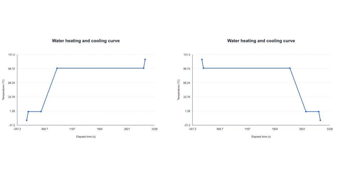
Introduce phase-change plateaus
Show a heating curve spanning ice, water and vapor in an introductory thermodynamics lesson. Constant-temperature segments distinguish latent heat from the temperature changes in each phase.
Explore this exampleFree Heating Curve of Water Generator Online
Explore an ideal constant-pressure water model with editable mass, temperatures and thermal parameters.
Water heating and cooling curve
Start with up to 150 free credits|No credit card required
Get up to 350 free credits on day one when you join through an invite.
Water heating and cooling curve
Calculate sensible heat and phase-change energy for water at 1 atm.
Ideal water model at 1 atm: fixed 0 °C and 100 °C transitions, constant heat capacities and power, and no heat loss. Latent heat is included only when the range strictly crosses a transition. At a boundary, the phase follows the interior of the selected temperature interval. Cooling uses positive transferred energy and elapsed time.
Calculated points: 6
Free Heating Curve of Water Generator Online— templates & examples
Updated
Free scientific tools
Explore an ideal constant-pressure water model with editable mass, temperatures and thermal parameters.
A heating curve of water relates transferred energy or time to temperature and phase changes. Explore an ideal constant-pressure water model with editable mass, temperatures and thermal parameters. Ice, water and vapor stages. Melting and boiling plateaus. Temperature range controls.
Ice, water and vapor stages. Melting and boiling plateaus. Temperature range controls.
Use an ideal water model at constant pressure to show sensible heating of ice, liquid water and vapor, with phase-change plateaus at 0°C and 100°C. A temperature range crossing both transitions includes the corresponding fusion and vaporization energies.
Enter the sample mass, start and end temperatures, heat capacities and latent heats. Sensible segments use Q=mcΔT and transitions use Q=mL, so changes to the physical inputs are reflected in the calculated energy rather than in a decorative curve.
View temperature against transferred energy or elapsed time. Constant positive power sets duration through t=Q/P; cooling reverses the thermal path while reporting positive energy-transfer magnitude and duration for the selected range.
Download SVG or PNG for a thermodynamics lesson and CSV for the plotted points. JSON settings preserve the model inputs so a changed mass, temperature range or power can be compared with the original configuration.
Open the heating curve generator and choose the initial and final temperatures.
Open the heating curve generator and choose the initial and final temperatures. A rising range heats the sample; a falling range follows the corresponding cooling path through the same model.
Set mass and positive constant power, then adapt the heat capacities or latent heats when needed. The water example supplies the values used by the displayed ideal constant-pressure calculation.
Select the horizontal axis for the teaching question. The preview shows sensible temperature changes and any phase-change plateaus included by the selected temperature interval.
Export SVG or PNG for the figure and CSV for the calculated path. Save project JSON to reopen the thermal parameters and compare a different sample or heating power.
Show a heating curve spanning ice, water and vapor in an introductory thermodynamics lesson.
Show a heating curve spanning ice, water and vapor in an introductory thermodynamics lesson. Constant-temperature segments distinguish latent heat from the temperature changes in each phase.
Explore this example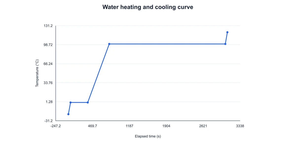
Change mass while keeping the temperature interval and material parameters fixed. The calculated curve gives a concrete comparison of energy required by different amounts of water.
Explore this example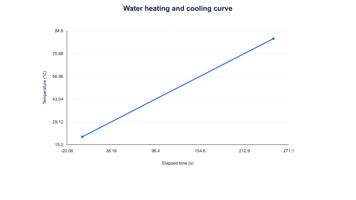
Use the time axis to discuss a constant-power heater. Keeping the thermal path fixed while changing power illustrates how the same energy transfer produces a different duration.
Explore this example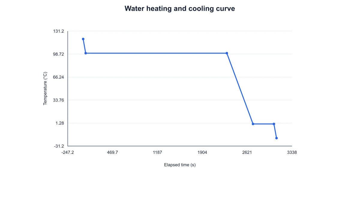
Create rising and falling temperature paths for the same endpoints. Positive transferred-energy magnitudes allow the two directions to be compared while the curve retains its thermal direction.
Explore this example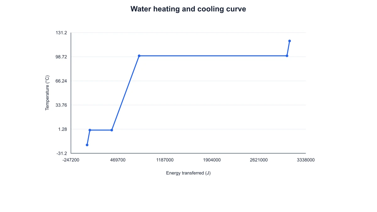
Export the plotted-point CSV alongside the figure in a worksheet. Students can connect the segment energies with Q=mcΔT and the phase transitions with Q=mL.
Explore this exampleSave JSON with the class model and its thermal constants. Another instructor can reopen the setup, vary a parameter and export a comparison curve for the next lesson.
Explore this exampleI used the heating curve of water to connect a temperature plot with the energy terms in our calculation. Setting the mass, endpoints and heater power produced a figure and a values table from one configuration. The exported SVG fitted the worked example, and CSV kept the segment values available beside it.
Bethany Scott
Physical chemistry lecturer · University of Durham
Free tools
A tool for every scientific figure
140 focused generators for the scientific figure you need — each opens in the right workspace with a matching example.
Illustrations, structures and concept diagrams
75 tools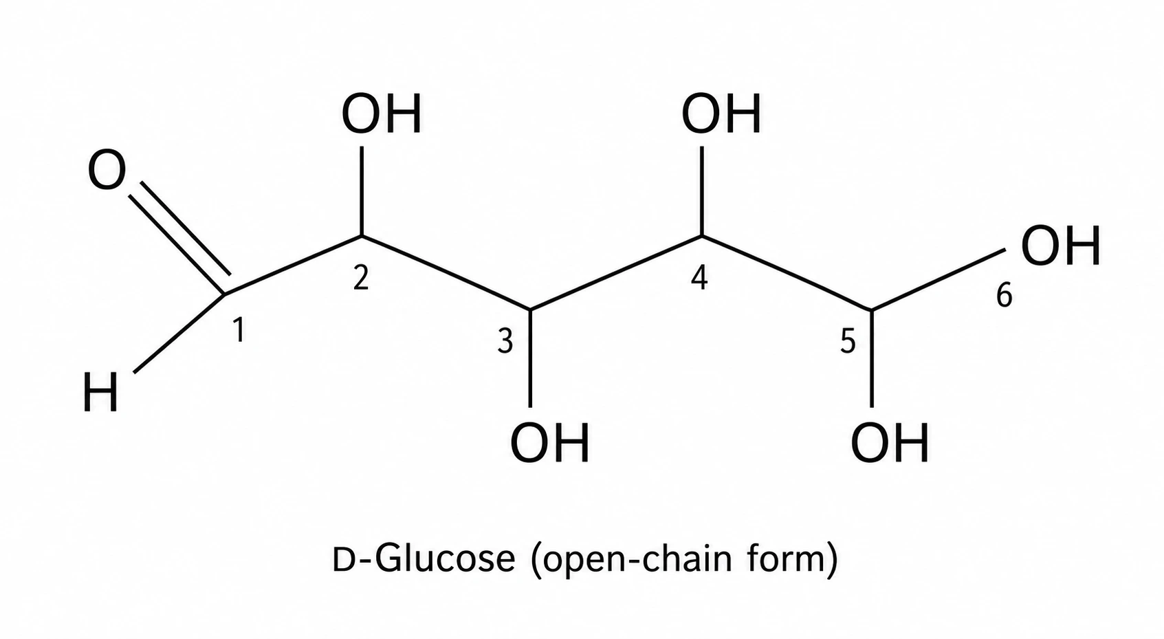 Chemistry Structure Generator
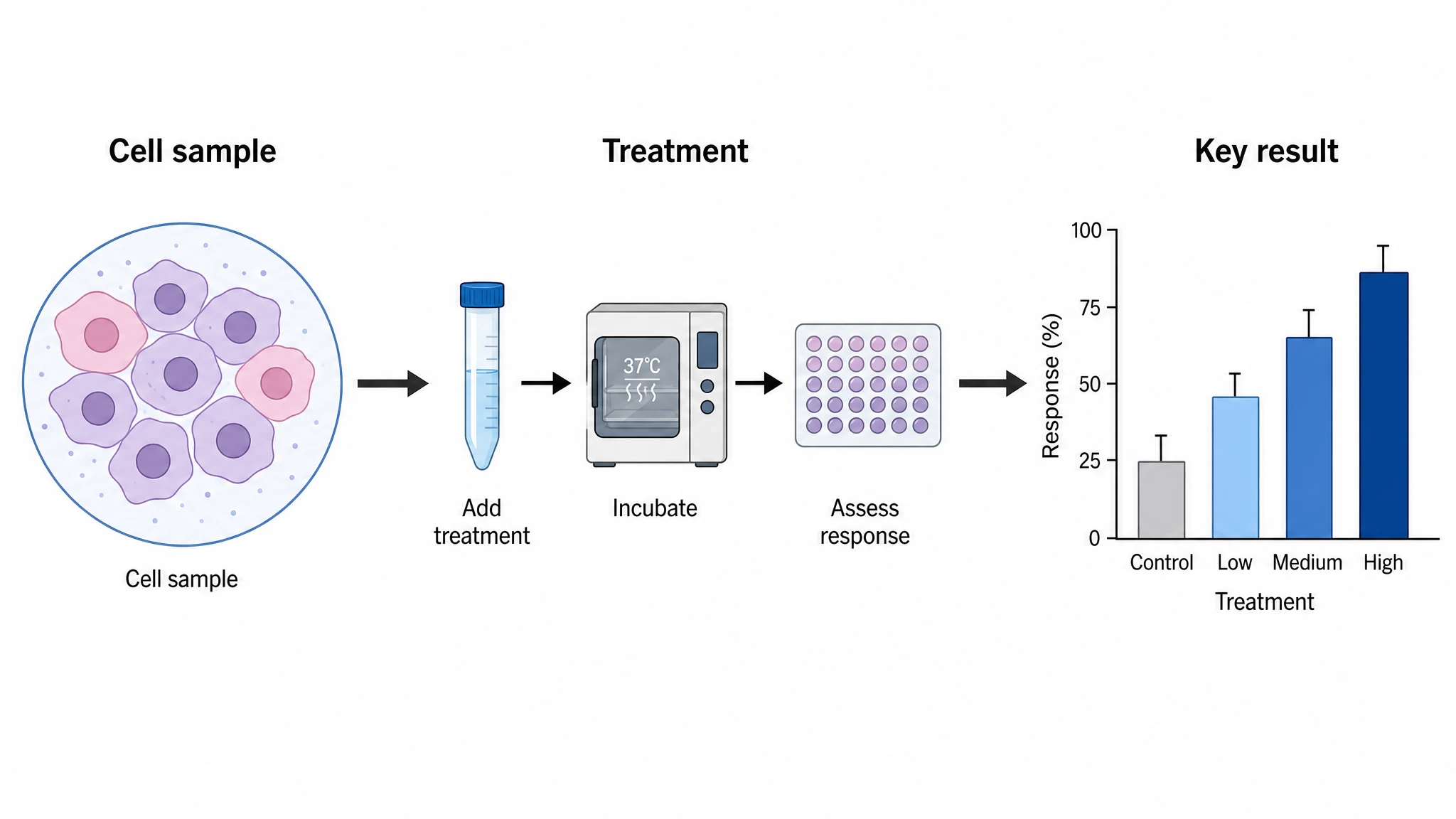 Graphical Abstract Maker
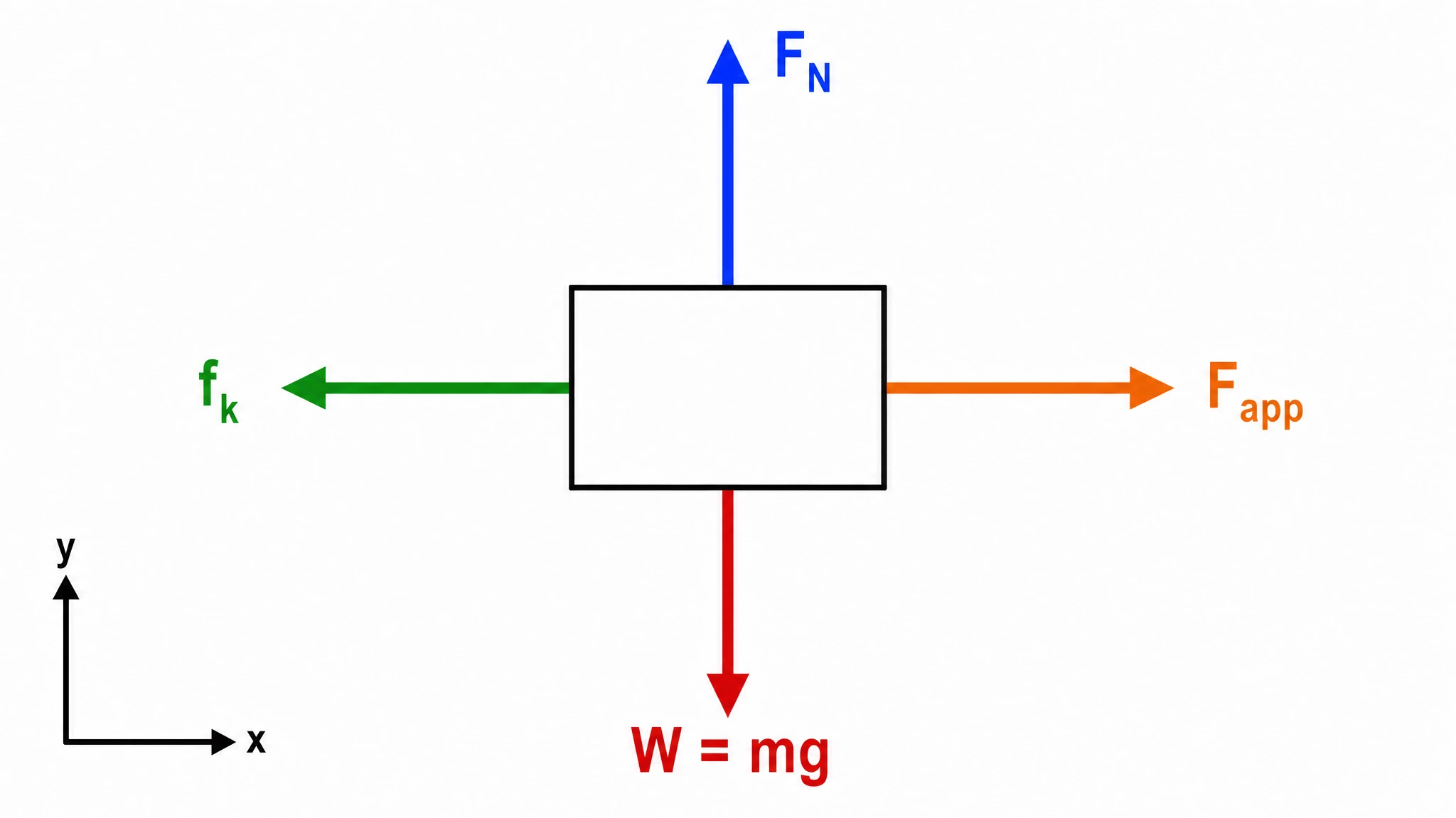 Free Body Diagram Generator
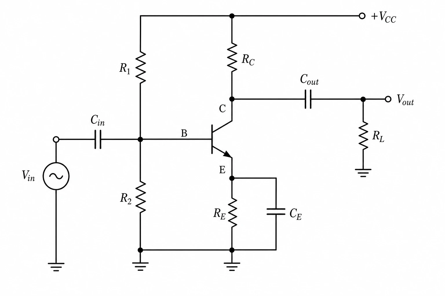 Circuit Diagram Maker
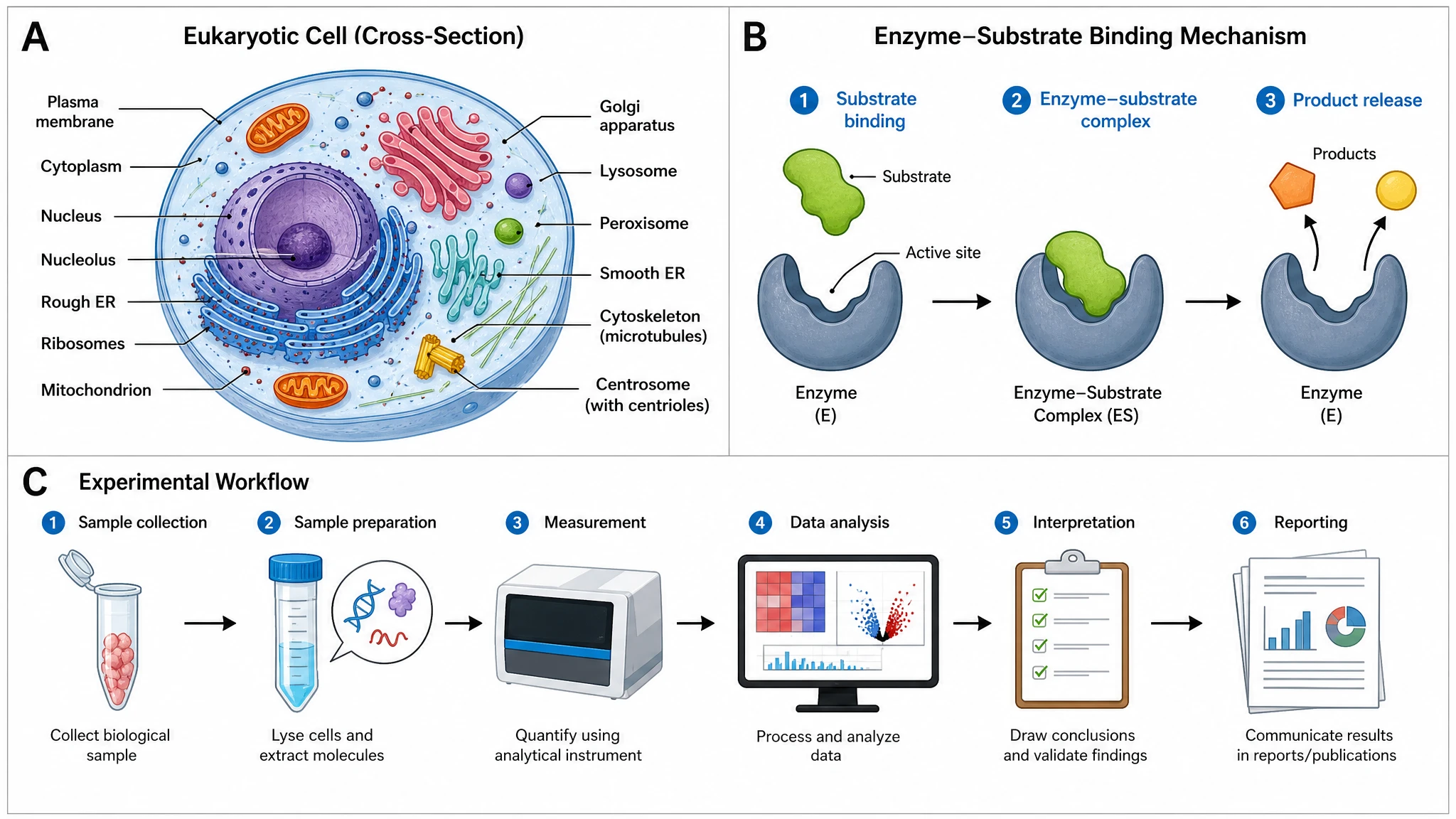 AI Scientific Image Generator
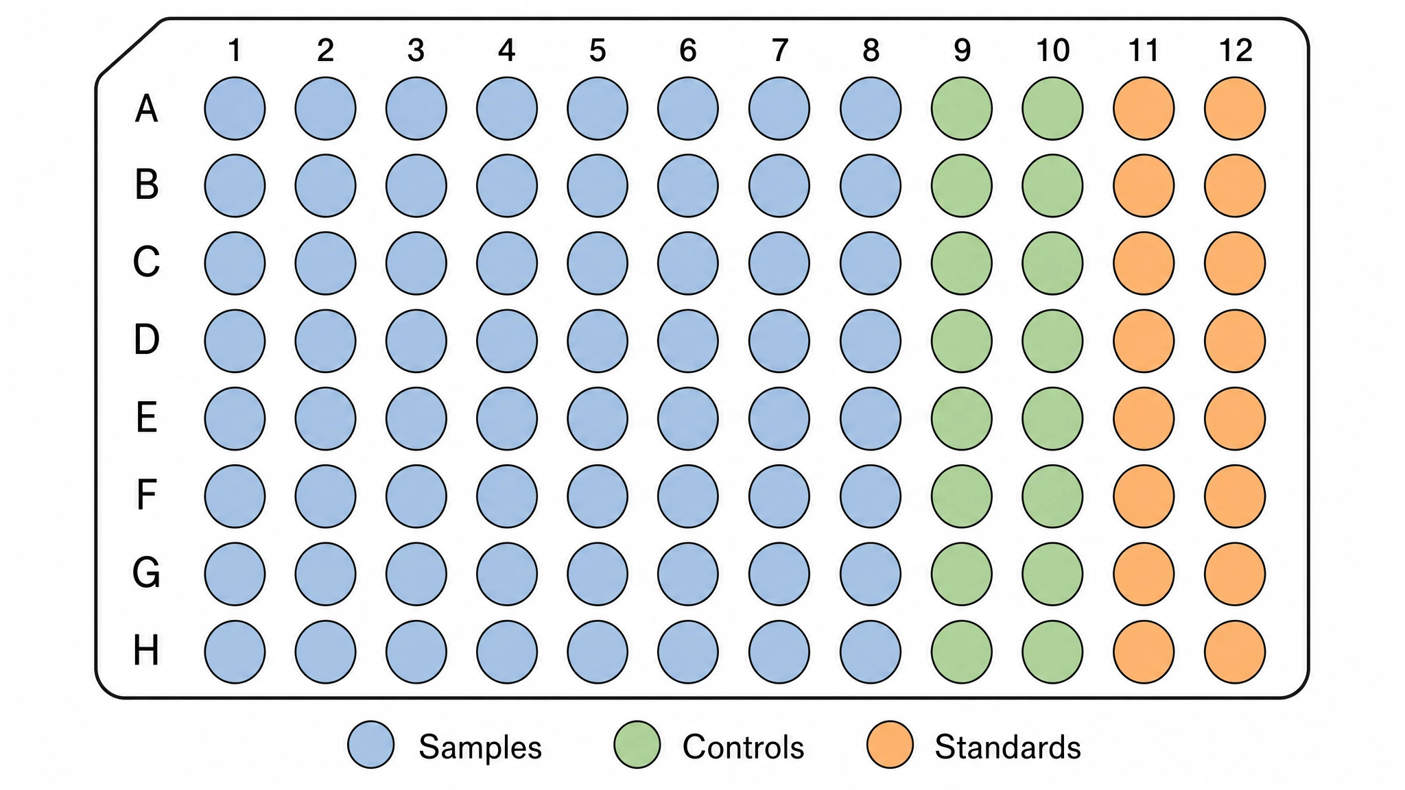 Editable 96-Well Plate
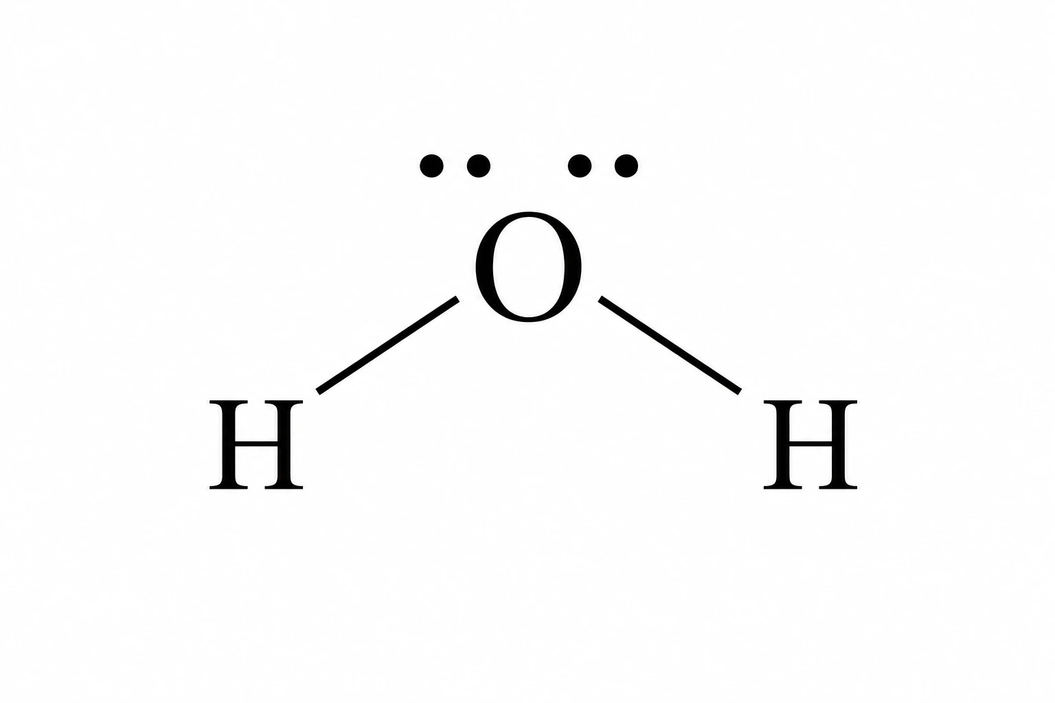 Lewis Dot Structure Generator
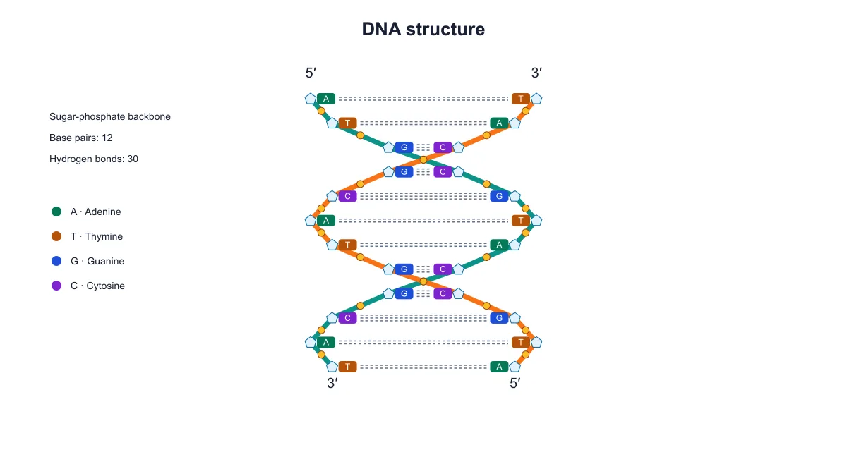 DNA Structure Diagram Generator
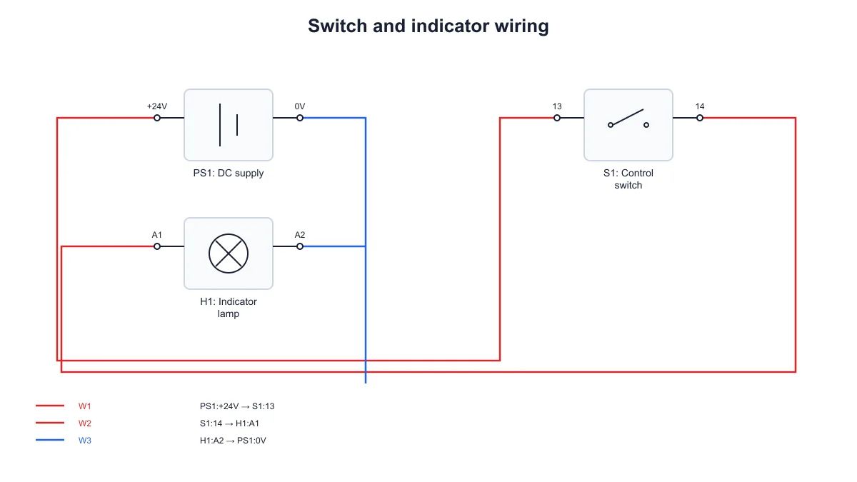 Wiring Diagram Maker
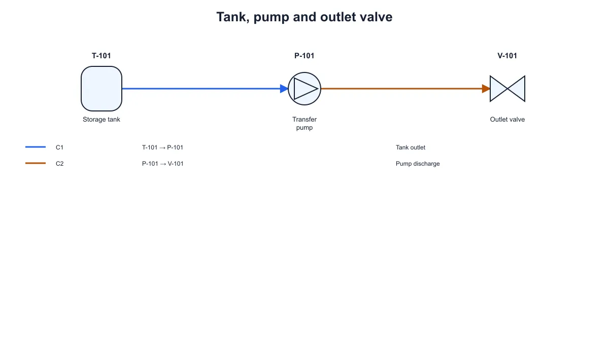 P&ID Diagram Generator
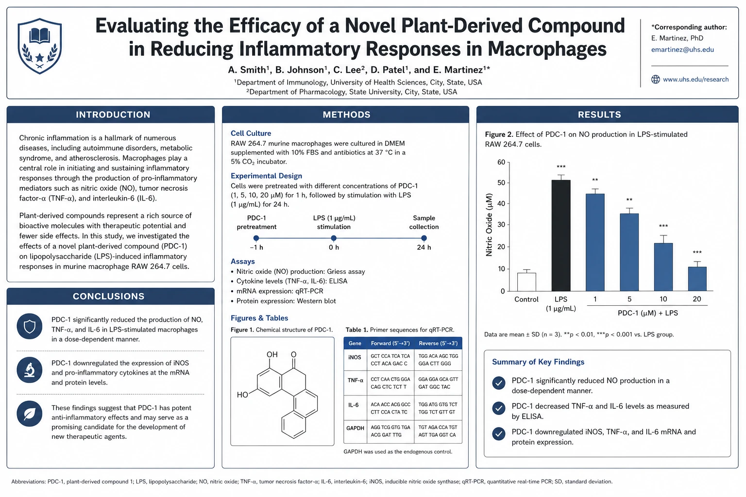 Scientific Poster Generator
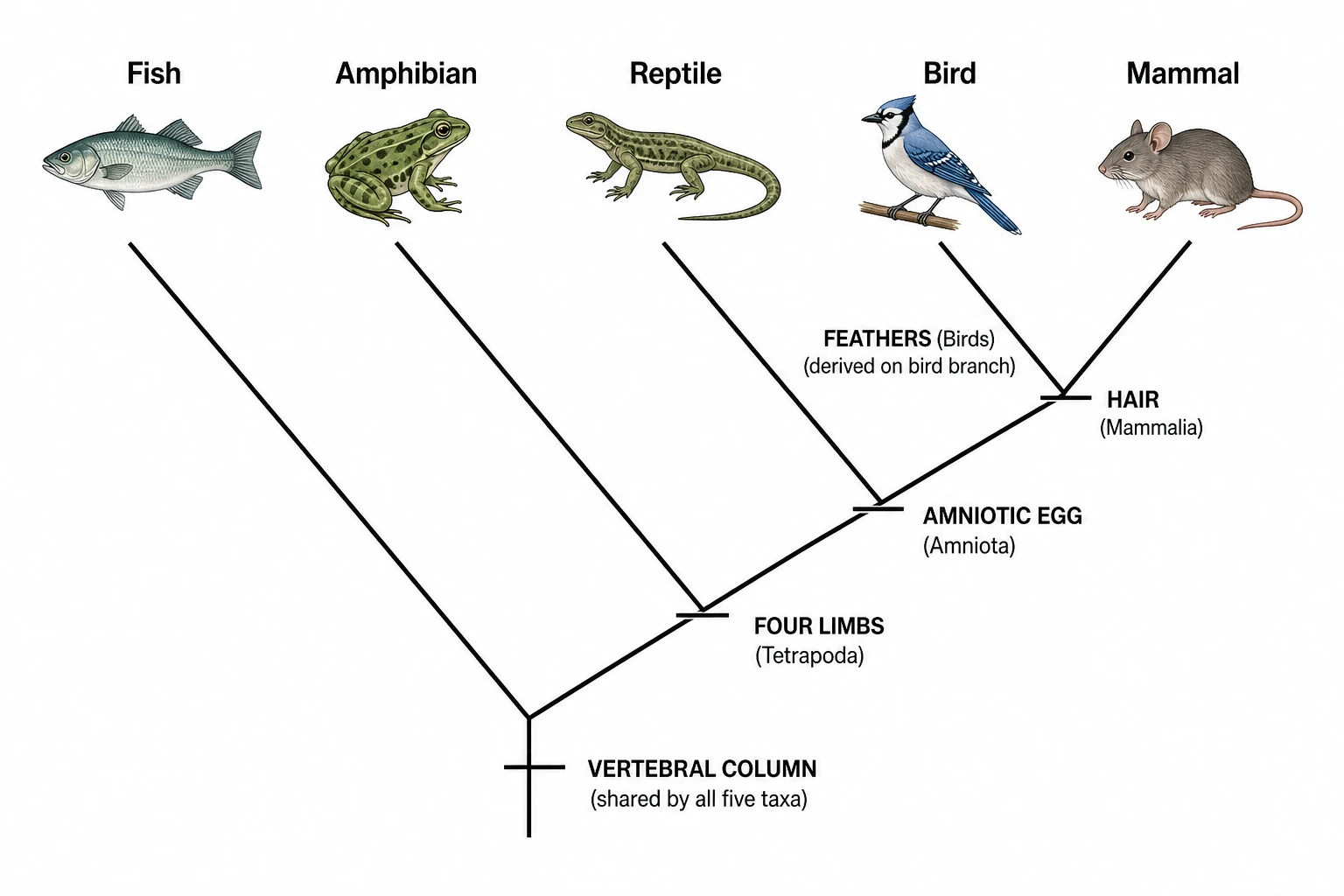 Cladogram Maker
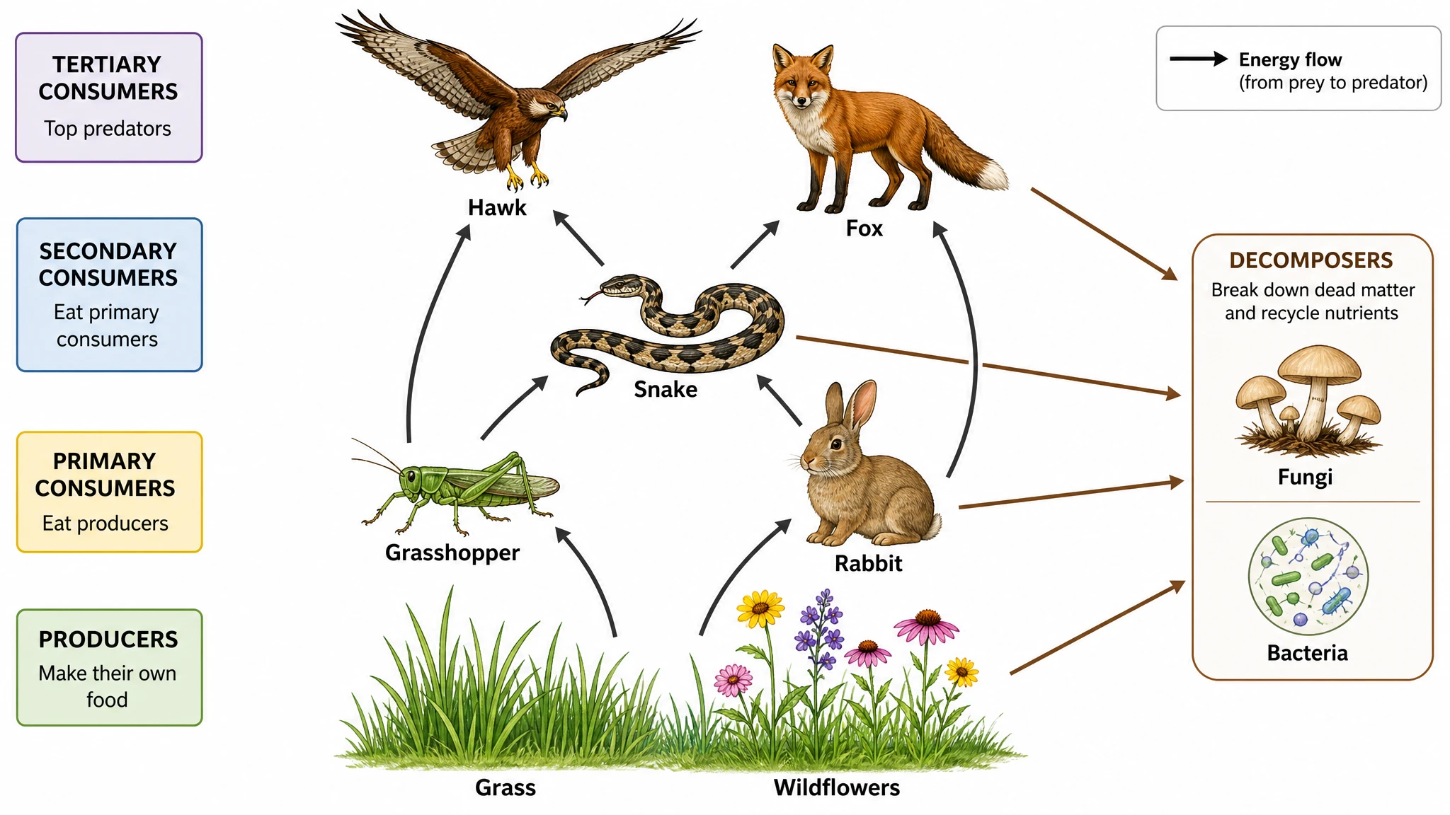 Food Web Maker
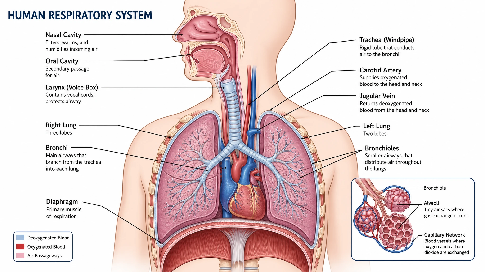 Medical Illustration Generator
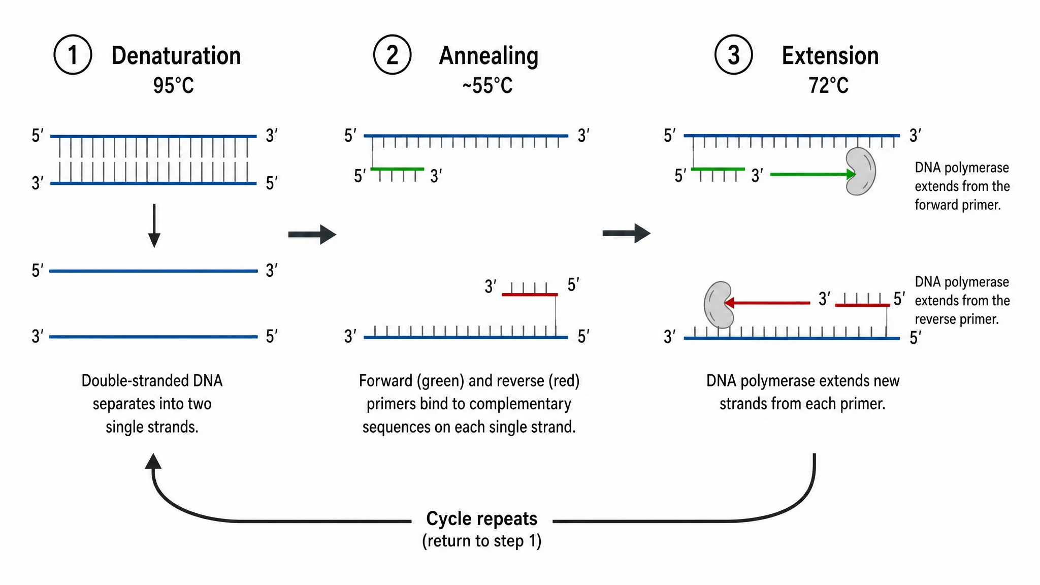 PCR Diagram Generator
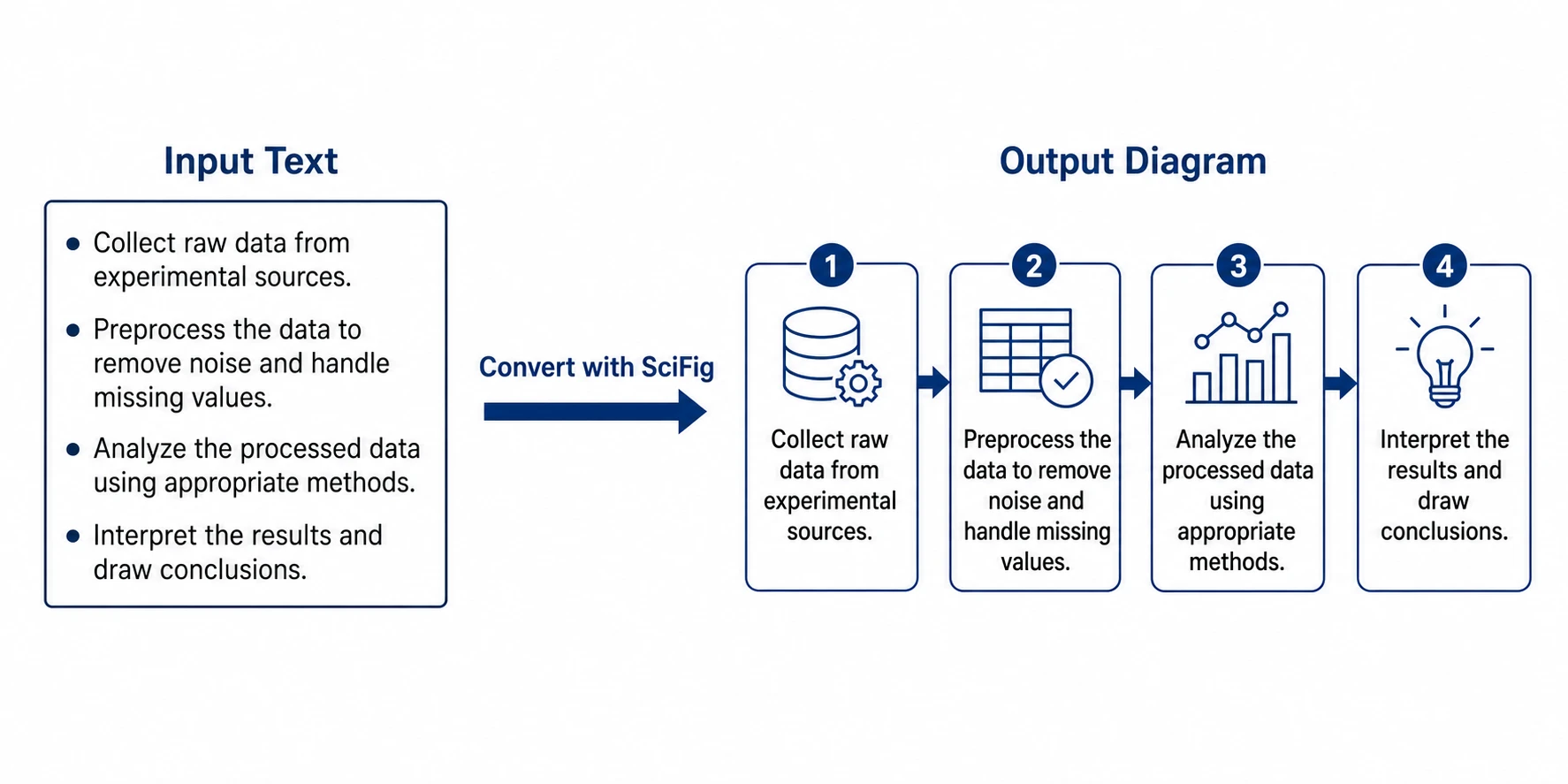 PPT Text to Visual Converter
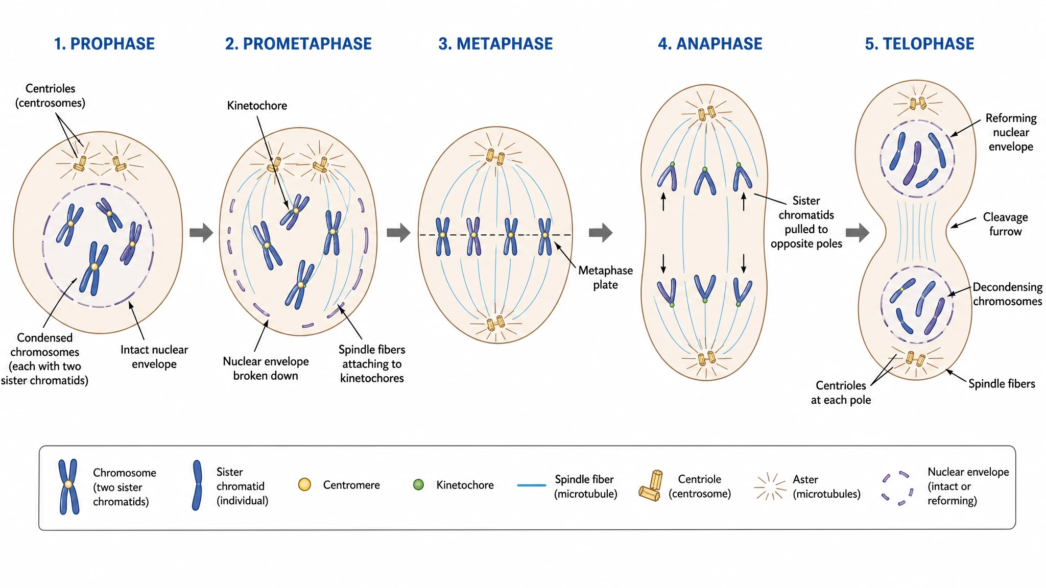 Mitosis Diagram Generator
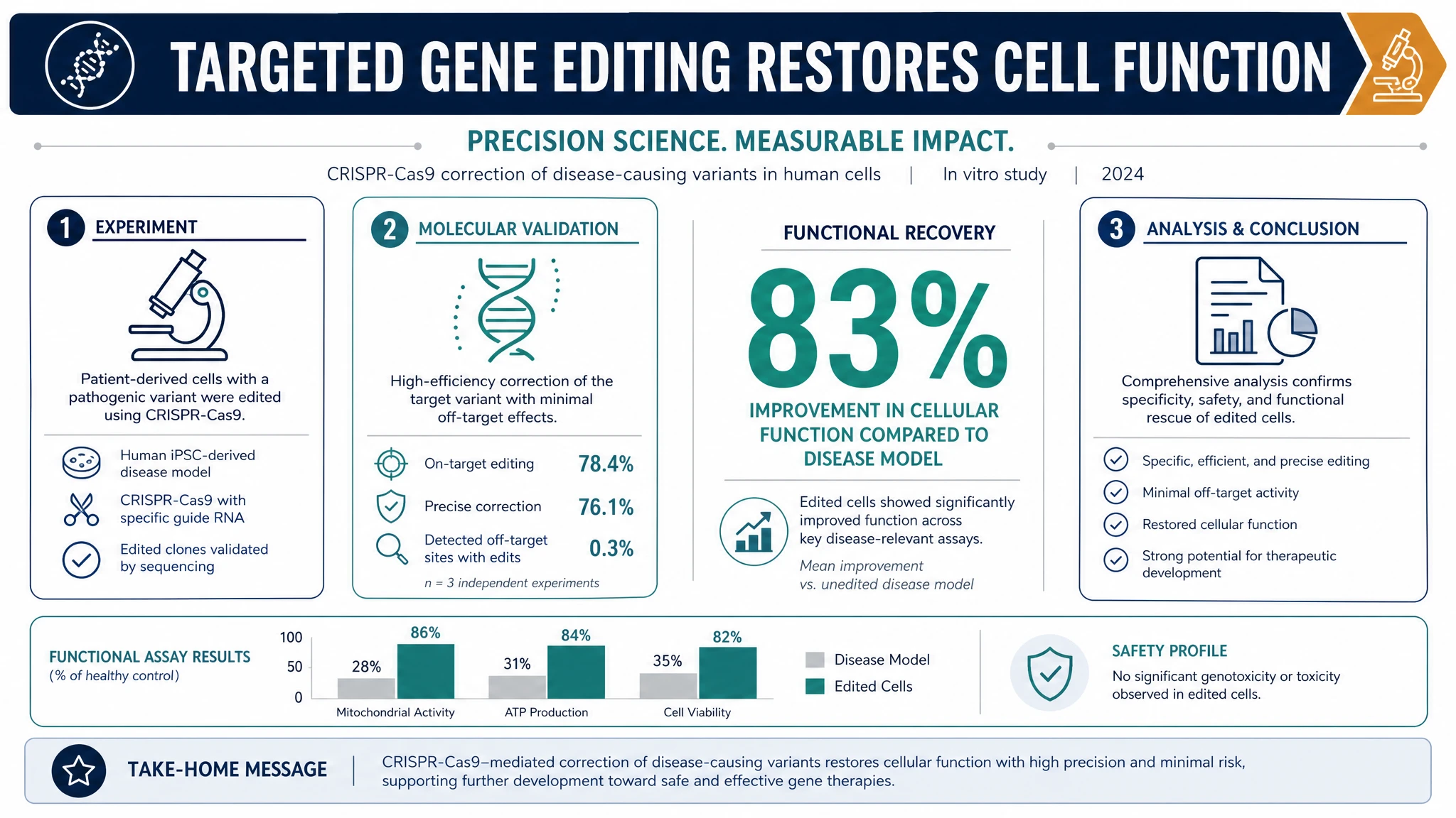 AI Infographic Generator
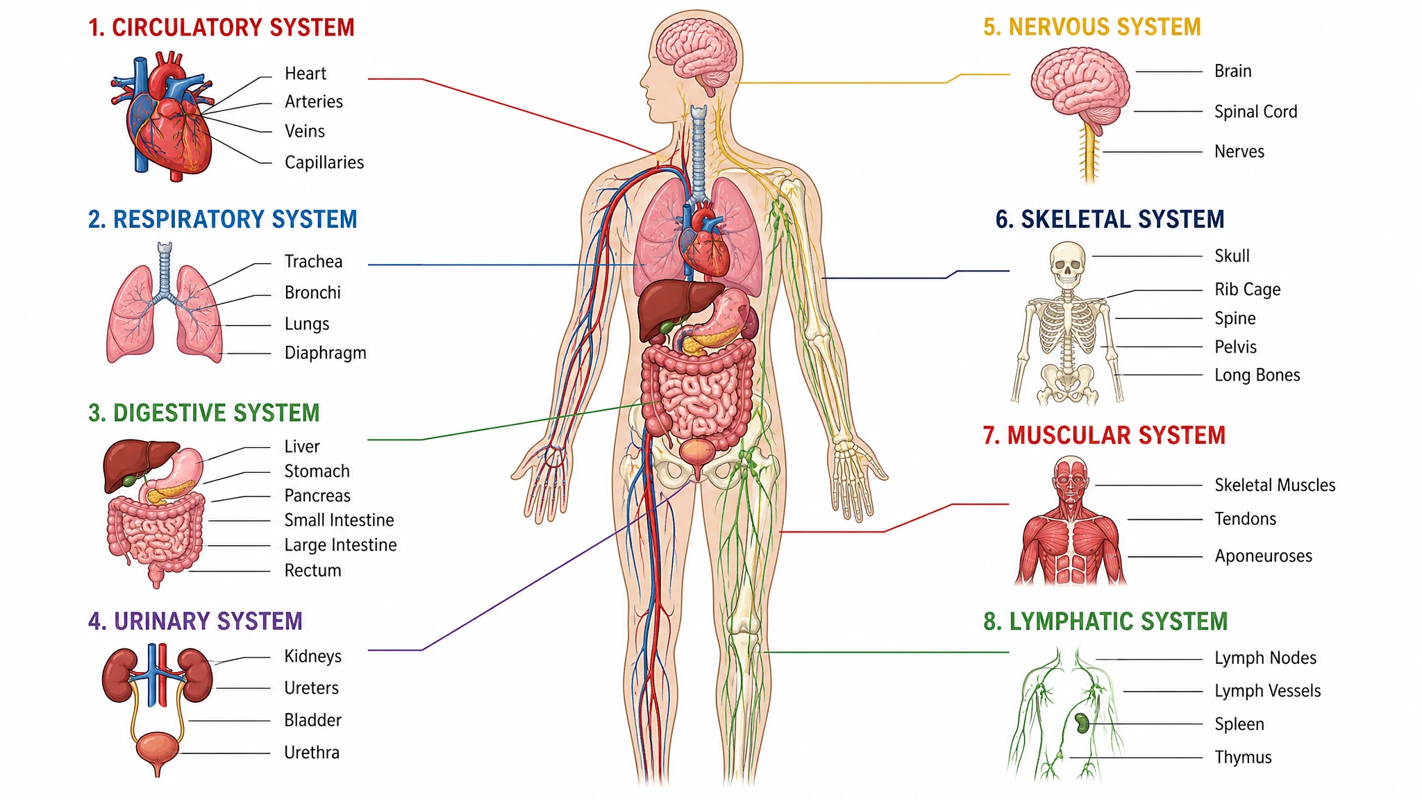 Anatomical Drawing Generator
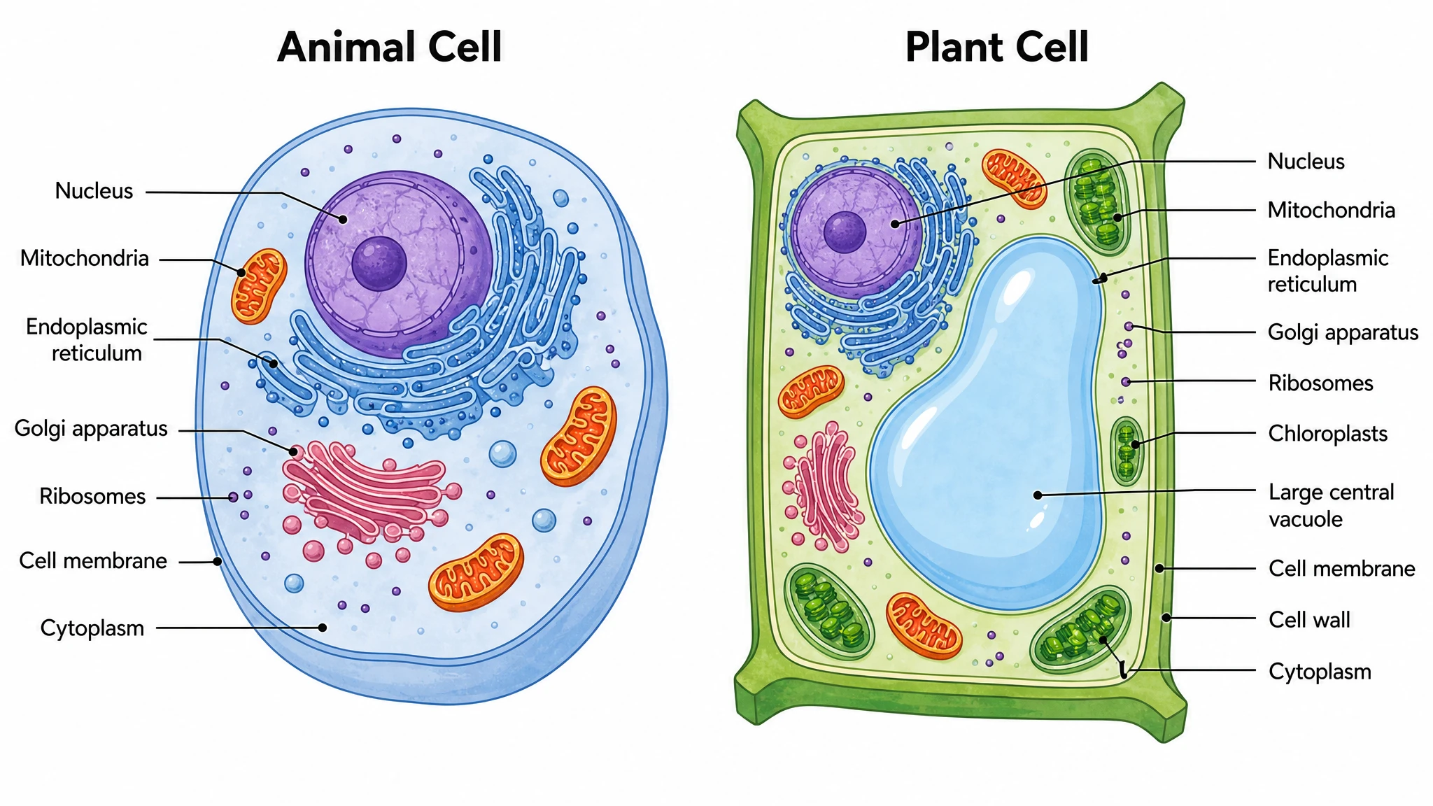 Animal and Plant Cell Comparison
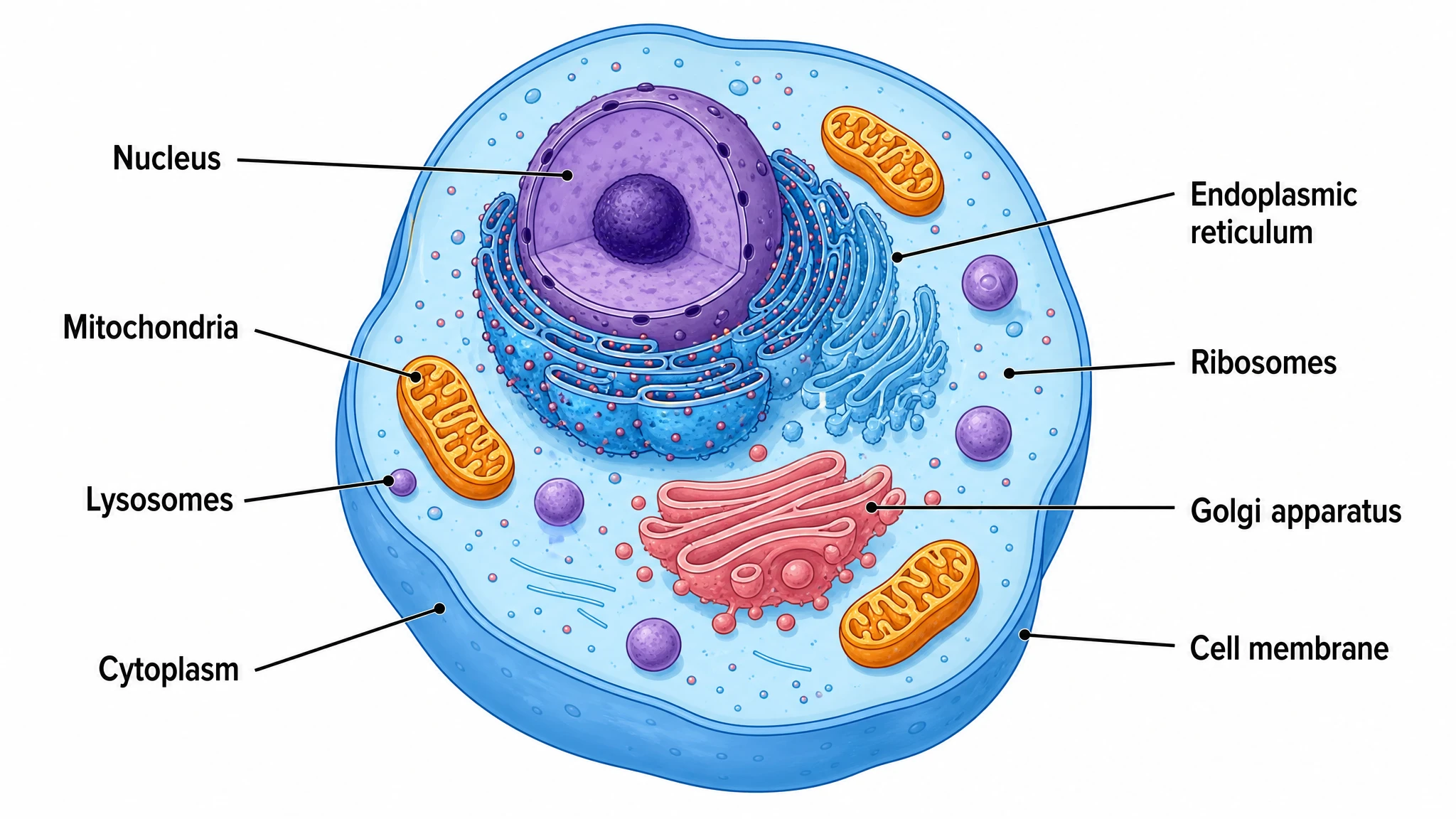 Animal Cell Diagram Generator
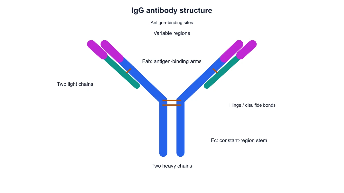 Antibody Structure Diagram Generator
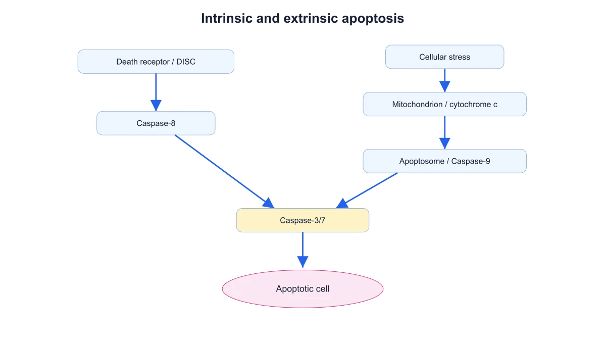 Apoptosis Diagram Generator
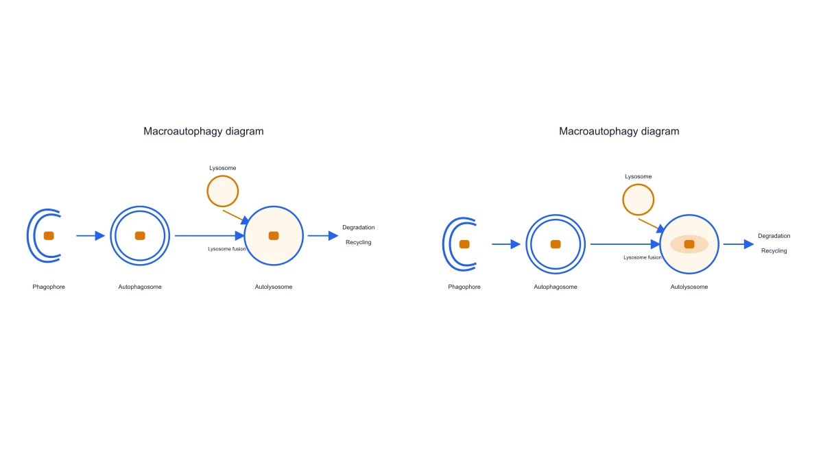 Autophagy Diagram Generator
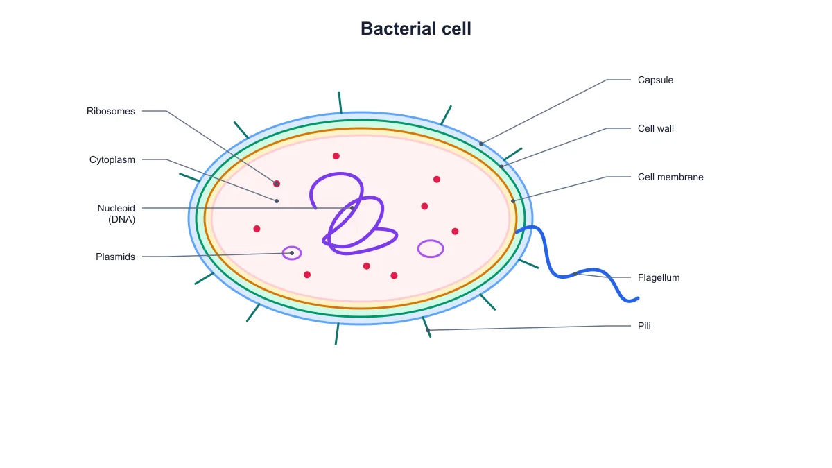 Bacteria Diagram Generator
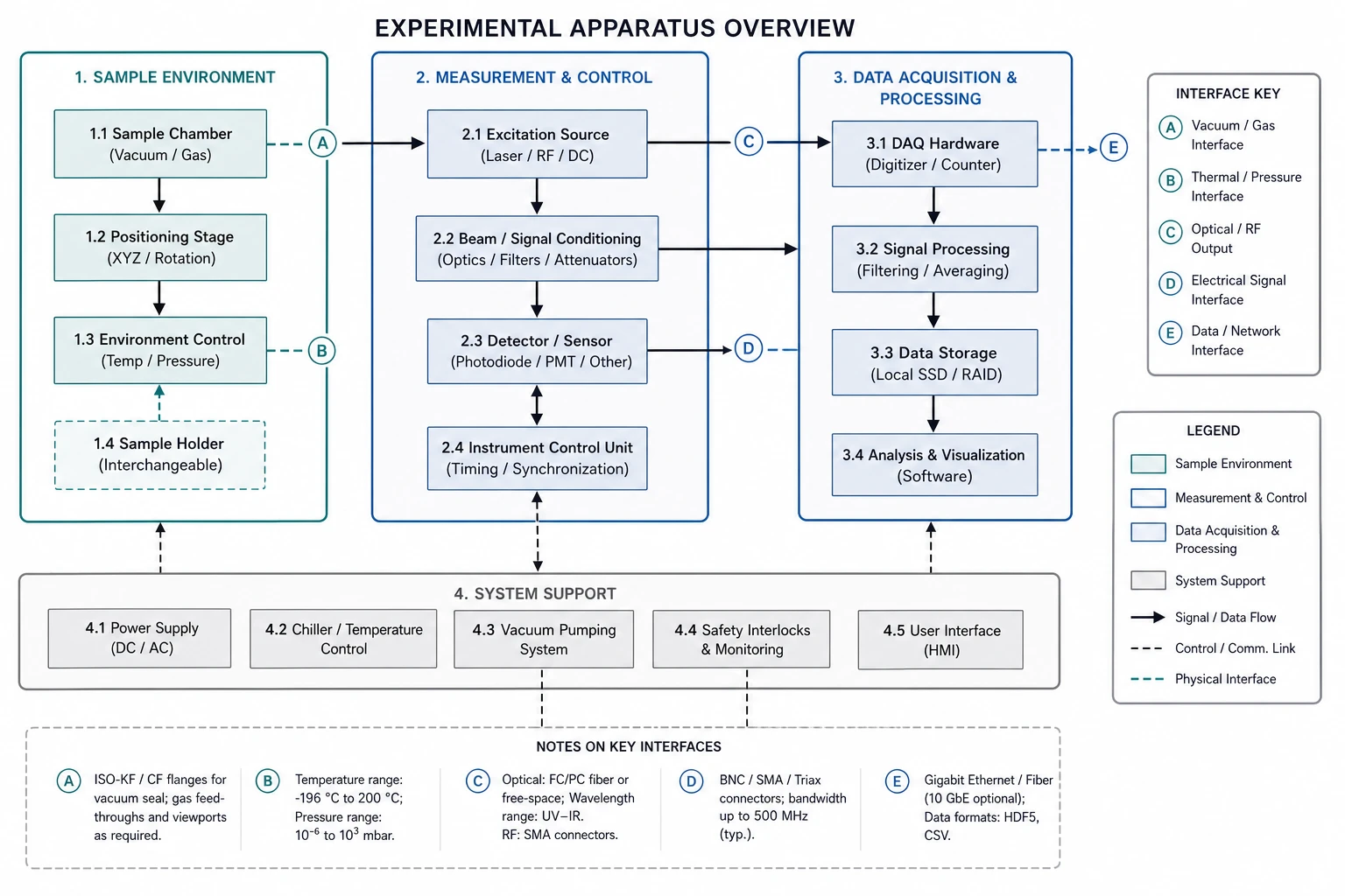 Blueprint Maker
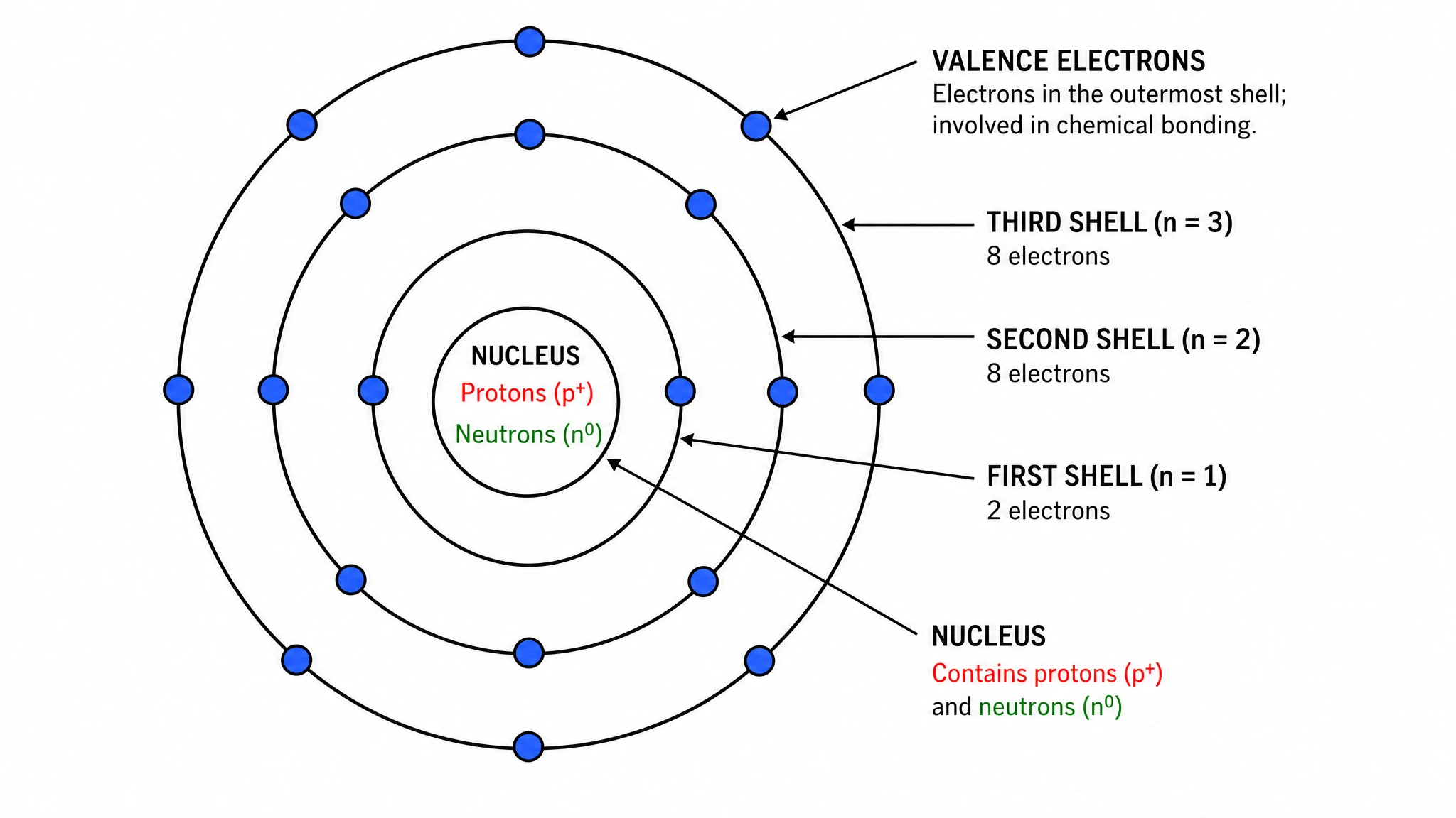 Bohr Model Maker
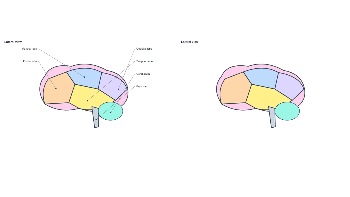 Brain Anatomy Diagram
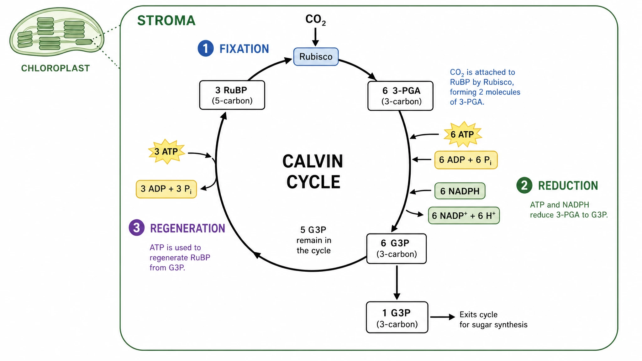 Calvin Cycle Diagram Generator
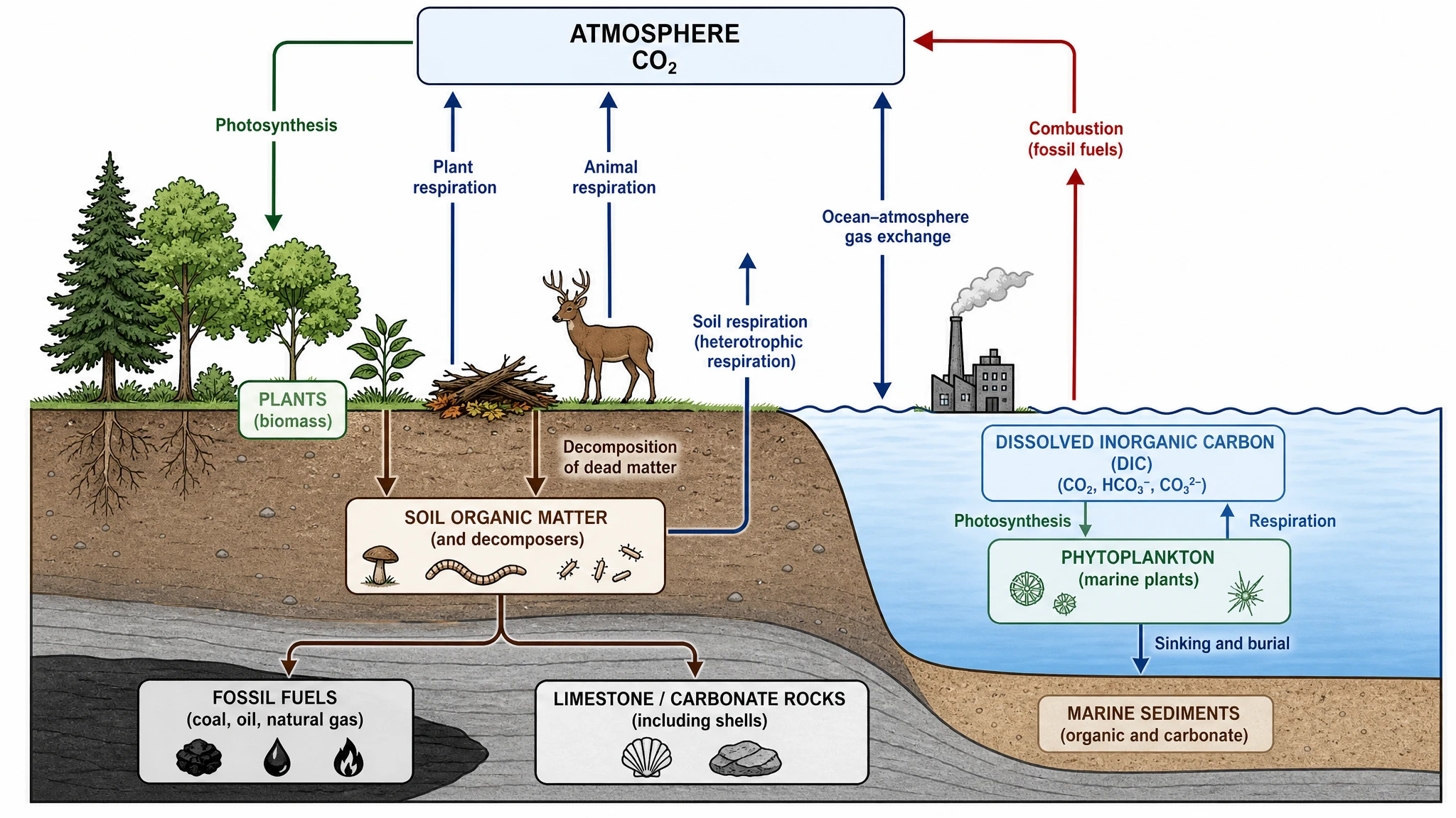 Carbon Cycle Diagram Generator
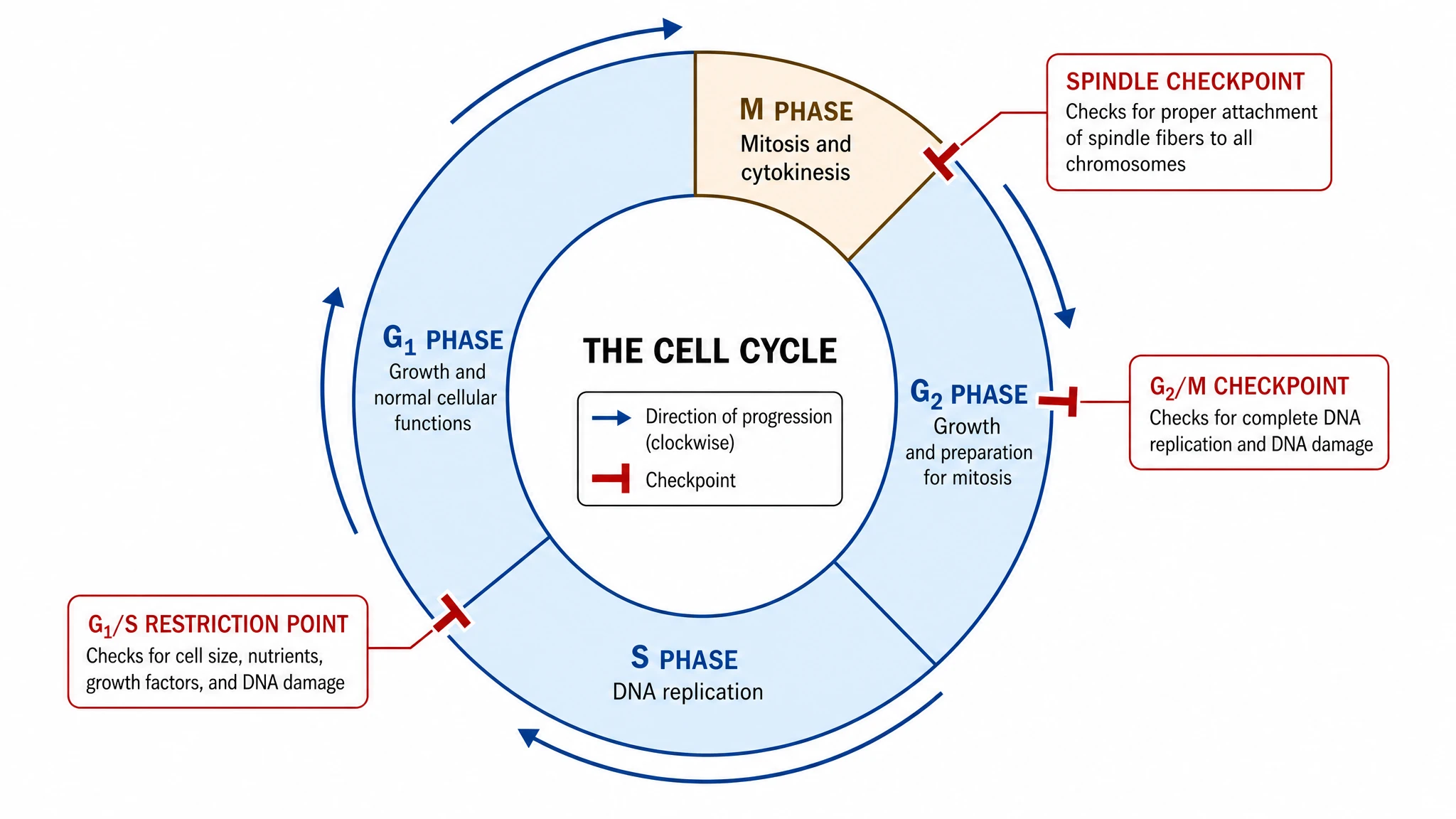 Cell Cycle Diagram Generator
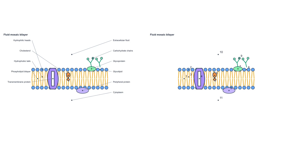 Cell Membrane Diagram
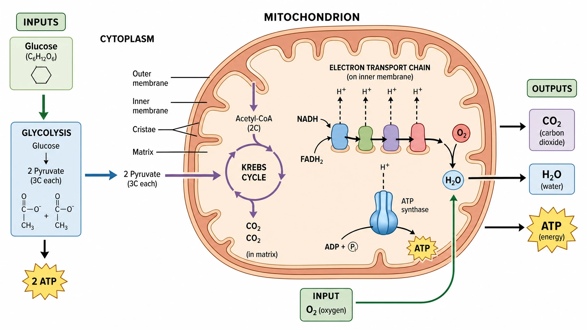 Cellular Respiration Diagram Generator
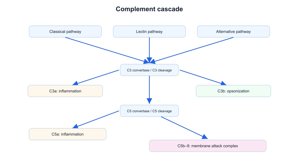 Complement System Diagram Generator
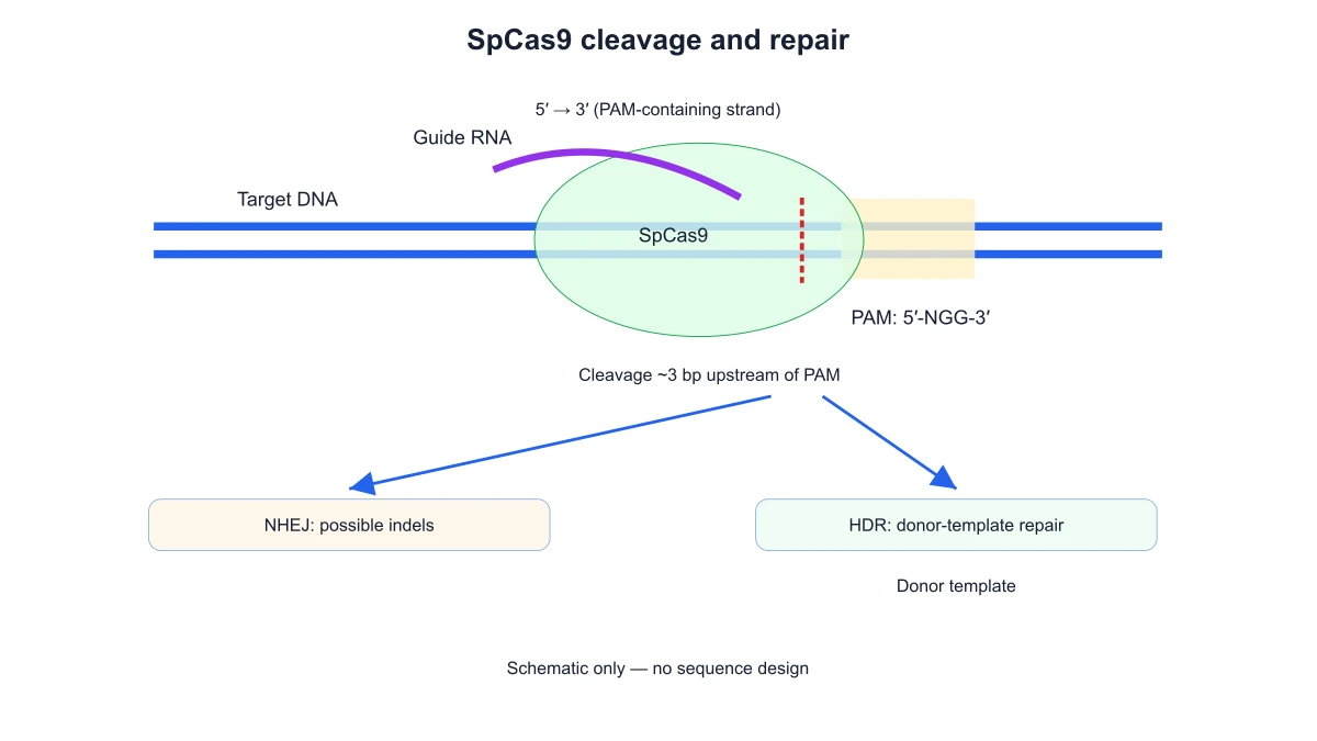 CRISPR-Cas9 Diagram Generator
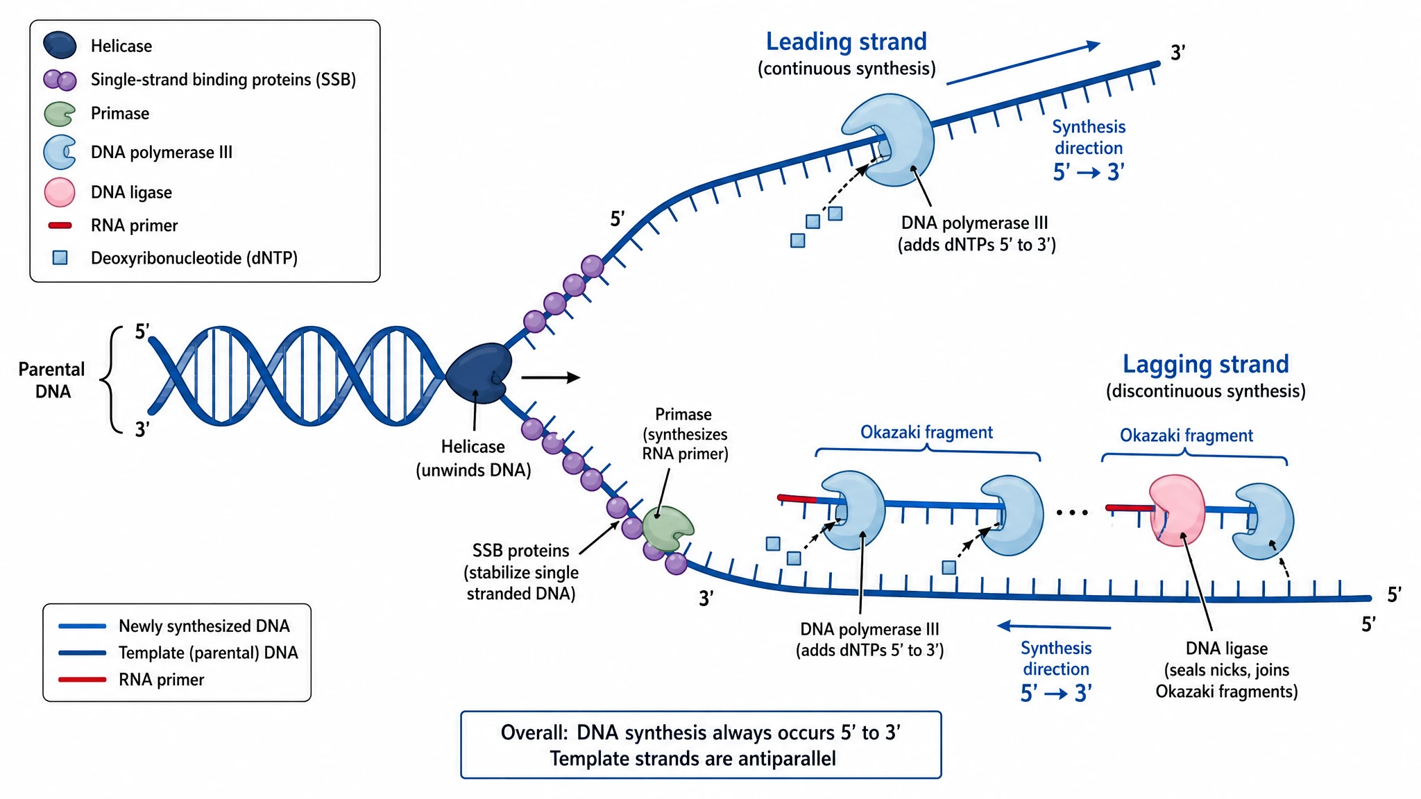 DNA Replication Diagram Generator
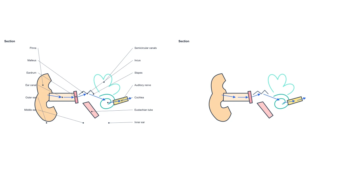 Ear Anatomy Diagram
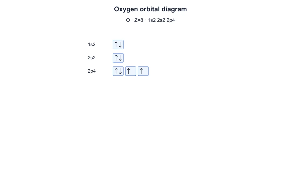 Electron Configuration Diagram Generator
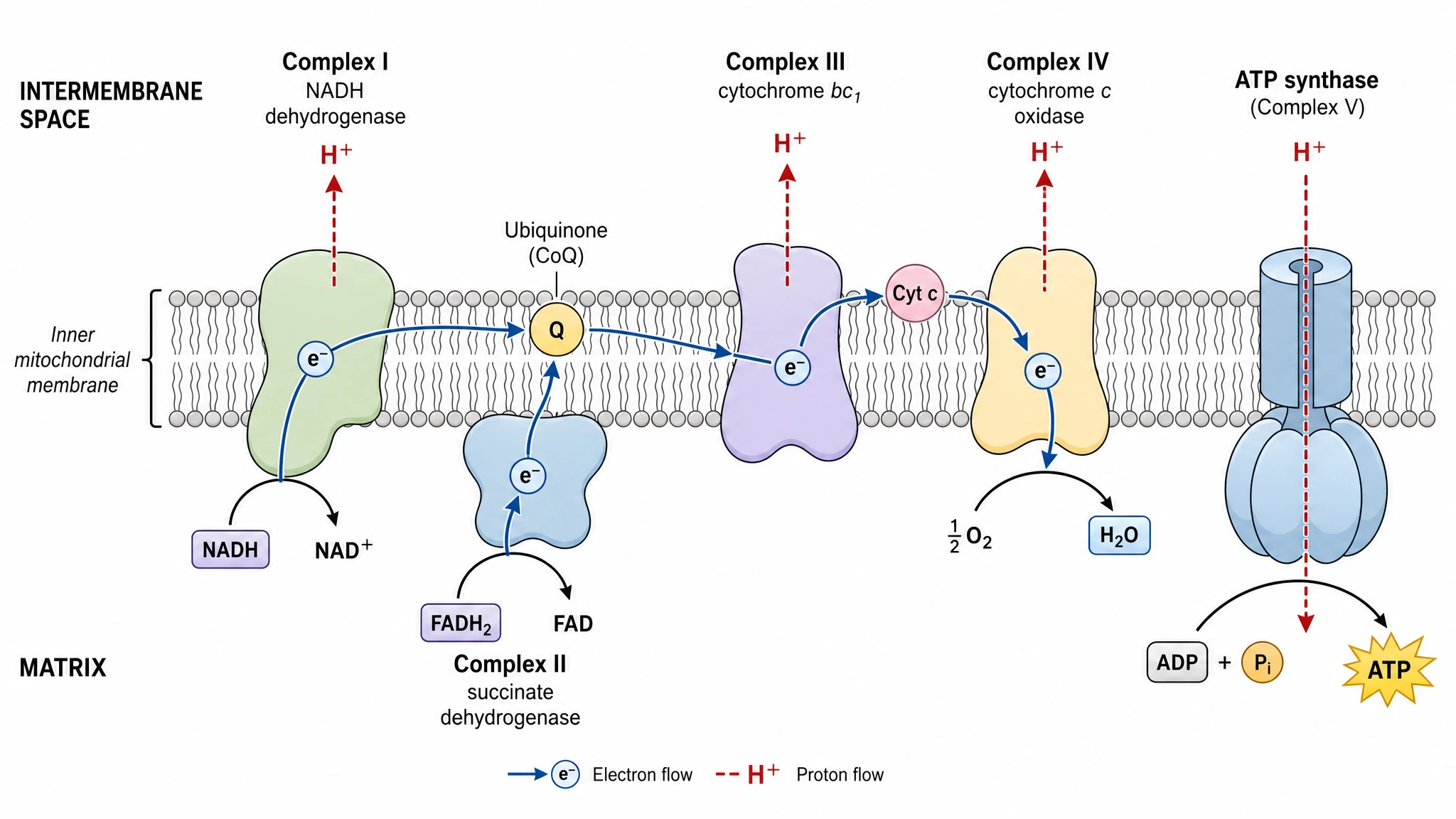 Electron Transport Chain Diagram Generator
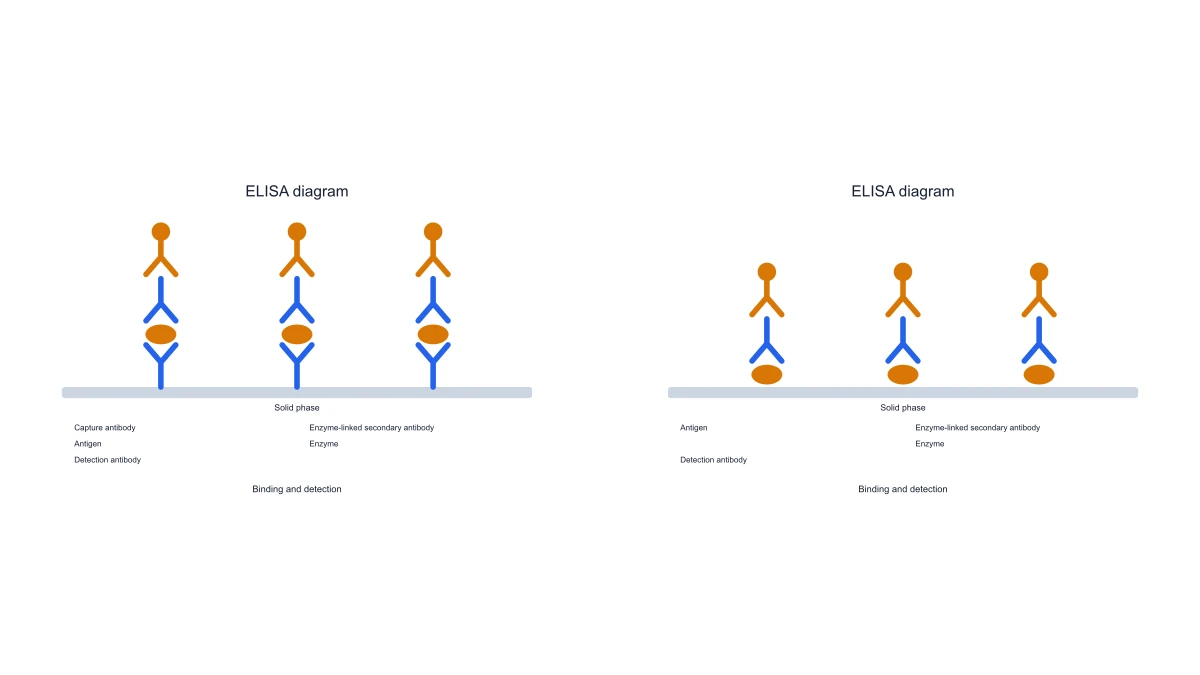 ELISA Diagram Generator
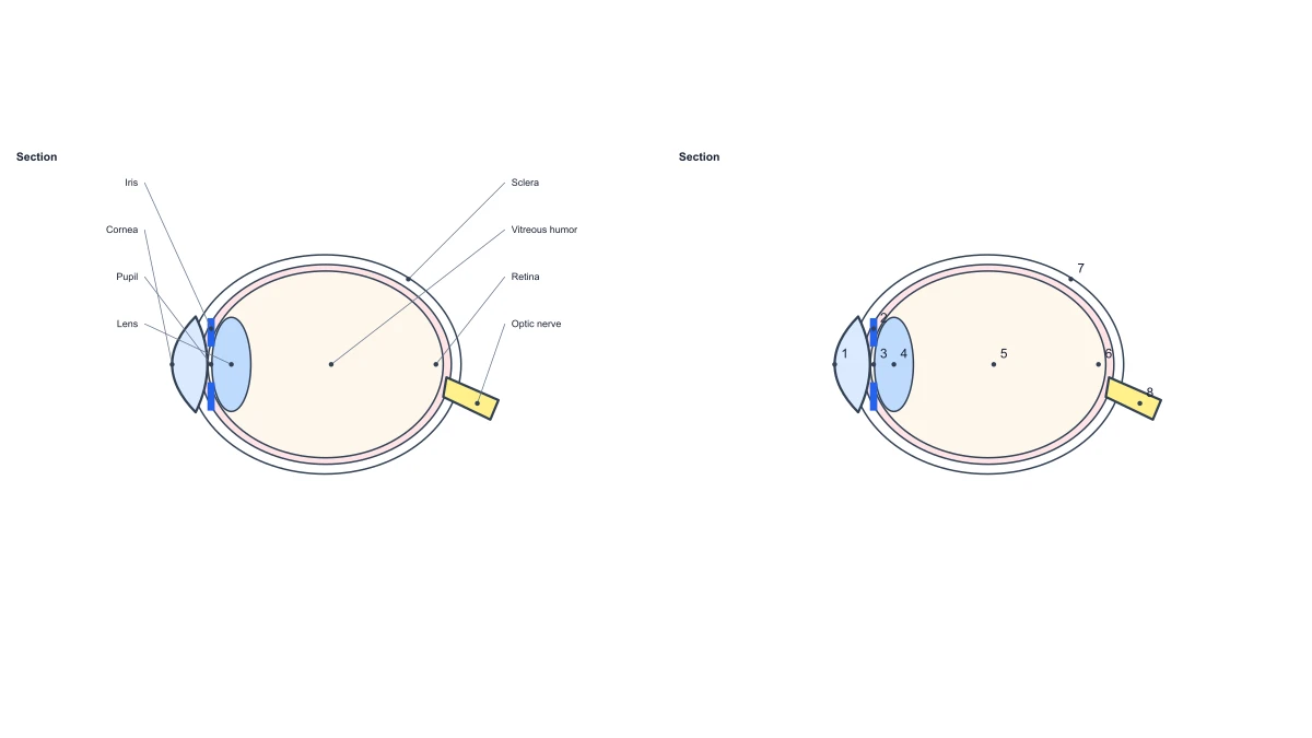 Eye Anatomy Diagram
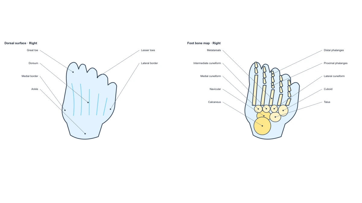 Foot Anatomy Diagram
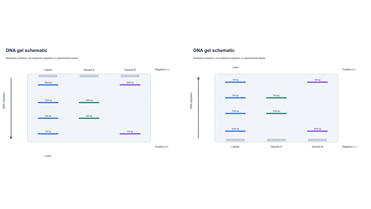 Gel Electrophoresis Diagram Generator
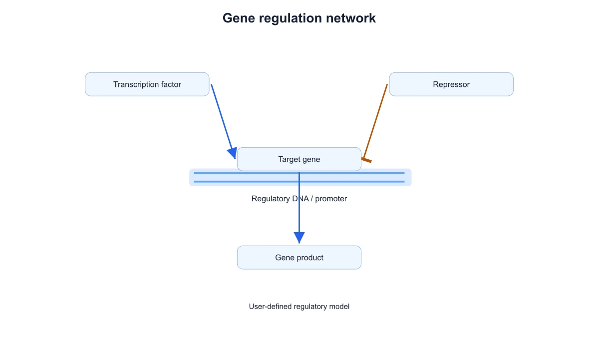 Gene Regulation Diagram Generator
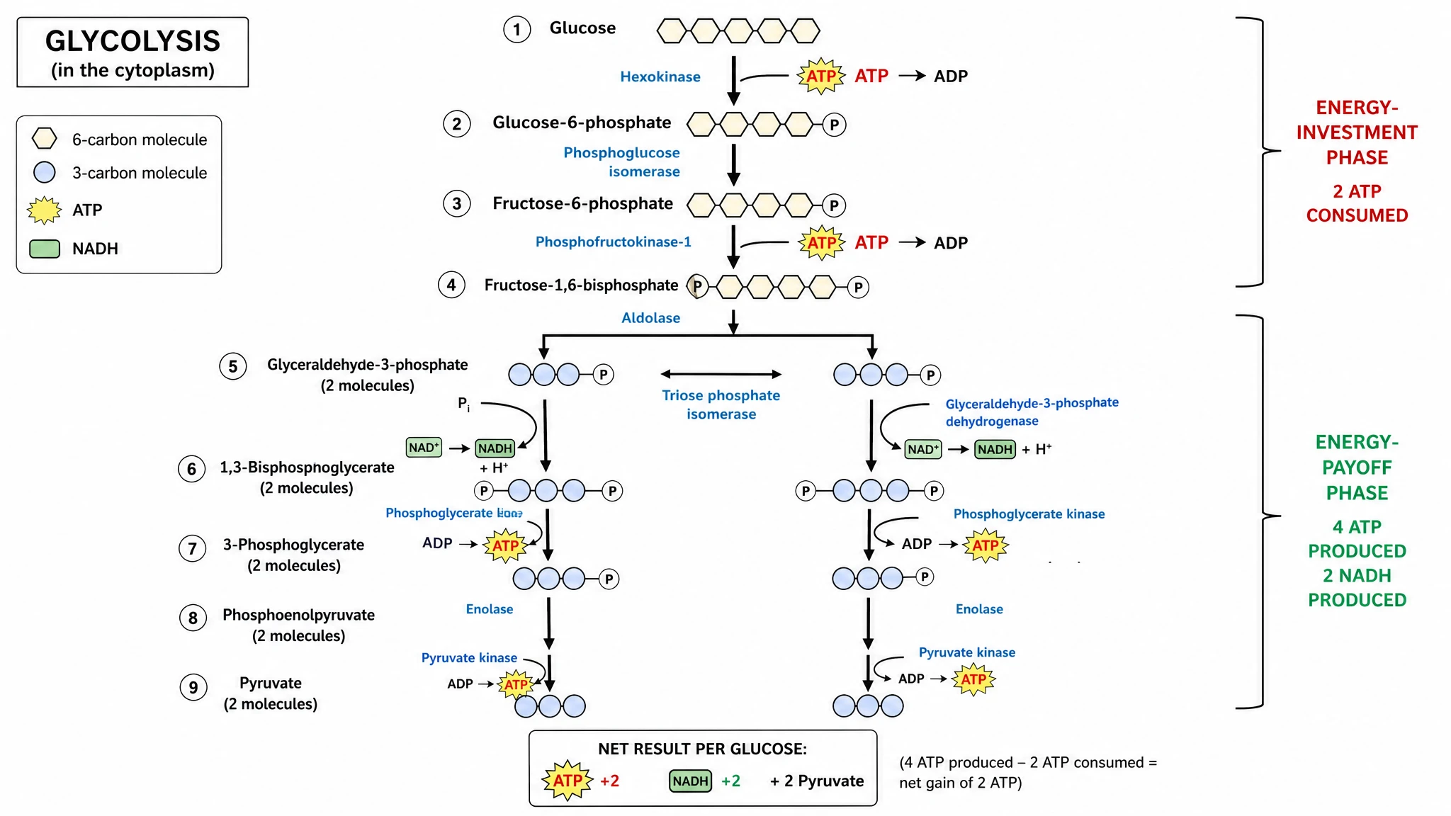 Glycolysis Diagram Generator
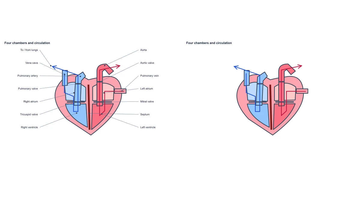 Heart Diagram
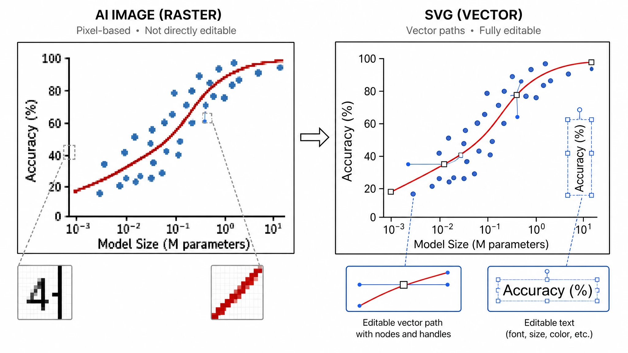 Image to Editable SVG Converter
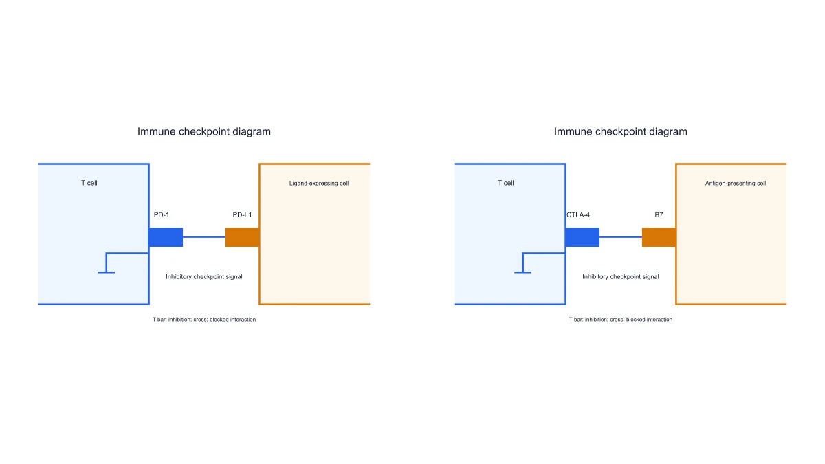 Immune Checkpoint Diagram Generator
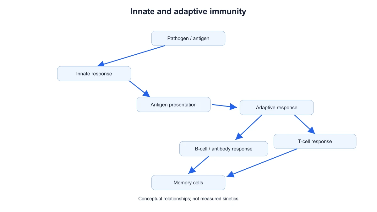 Immune Response Diagram Generator
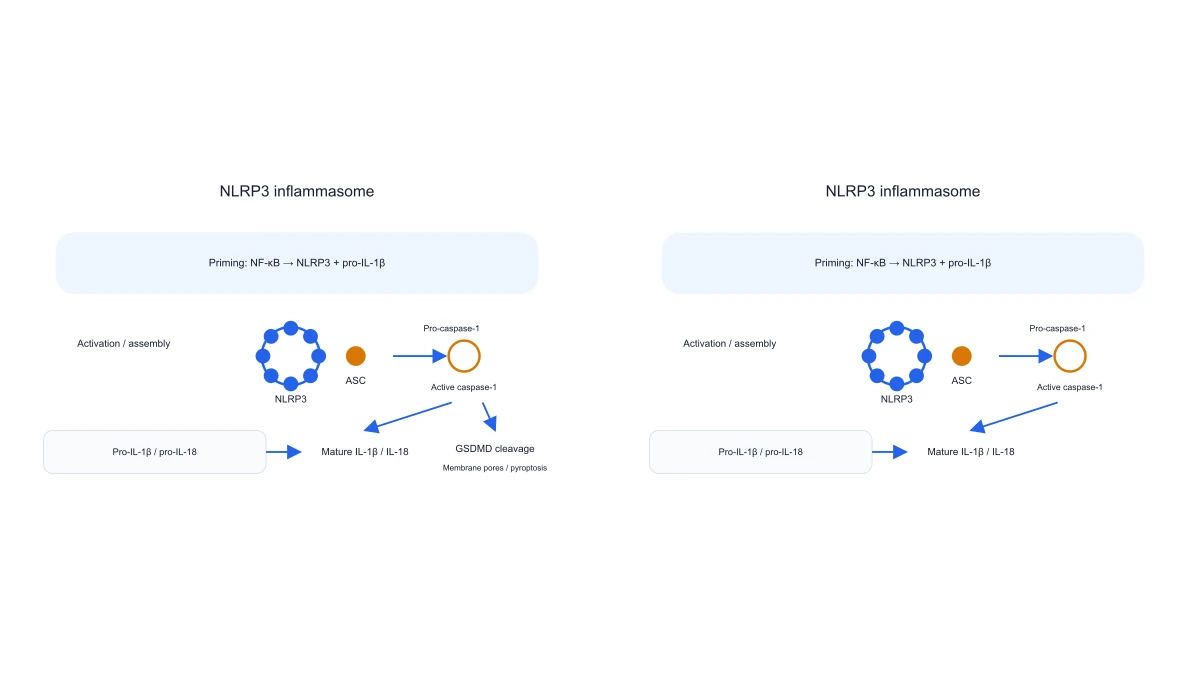 Inflammasome Diagram Generator
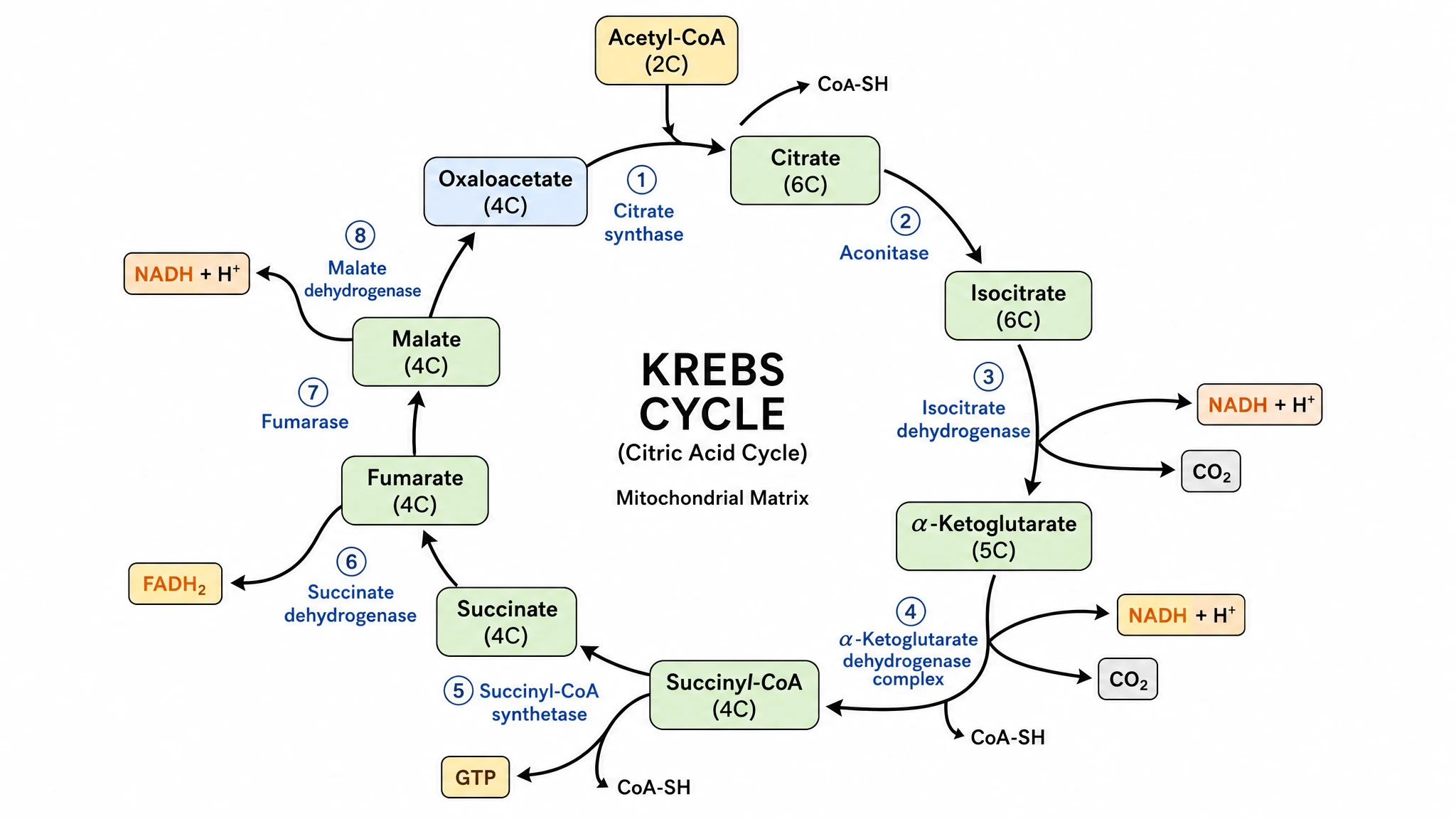 Krebs Cycle Diagram Generator
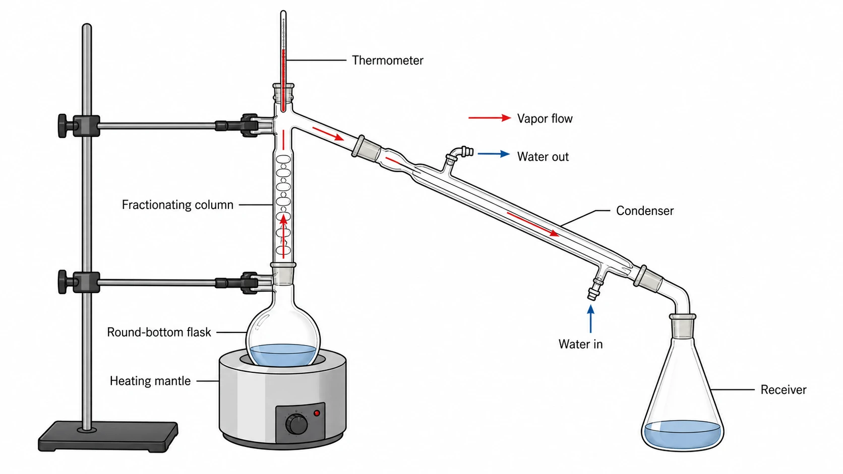 Lab Diagram Maker
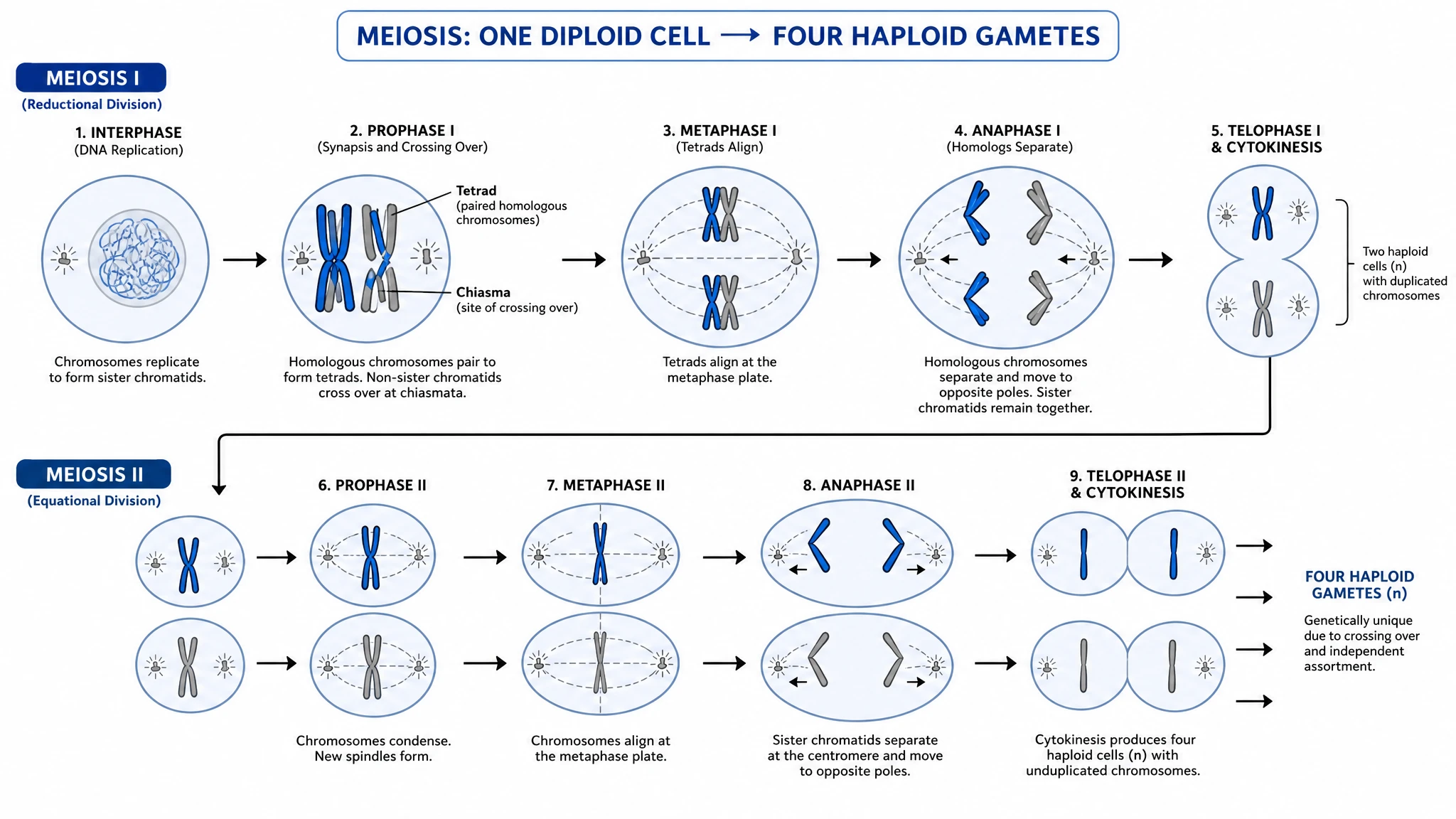 Meiosis Diagram Generator
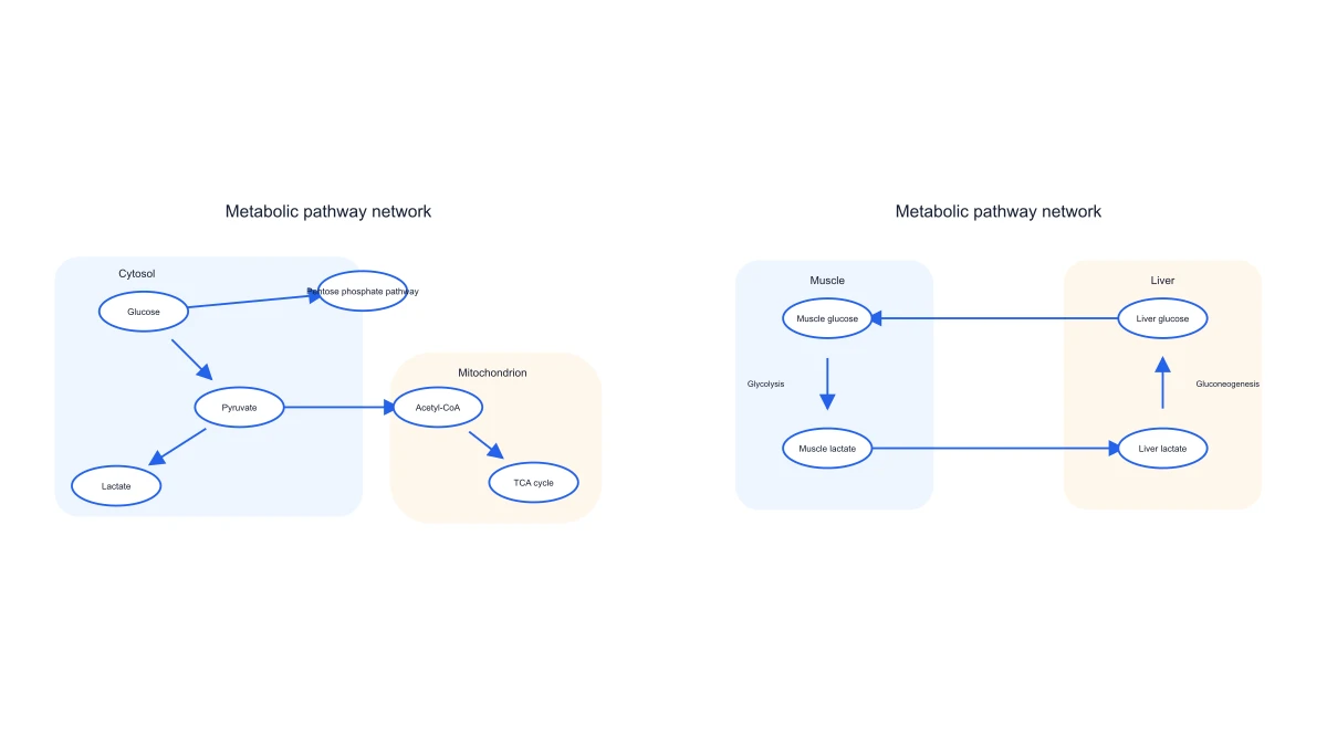 Metabolic Pathway Diagram Generator
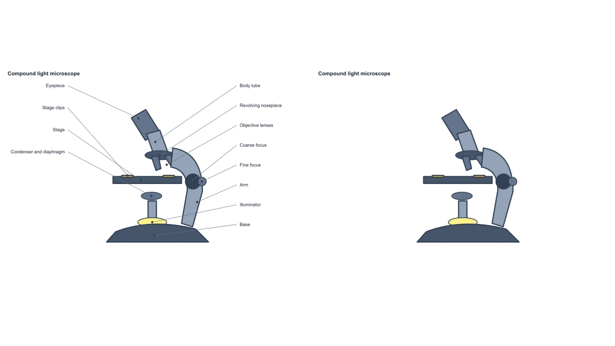 Microscope Diagram
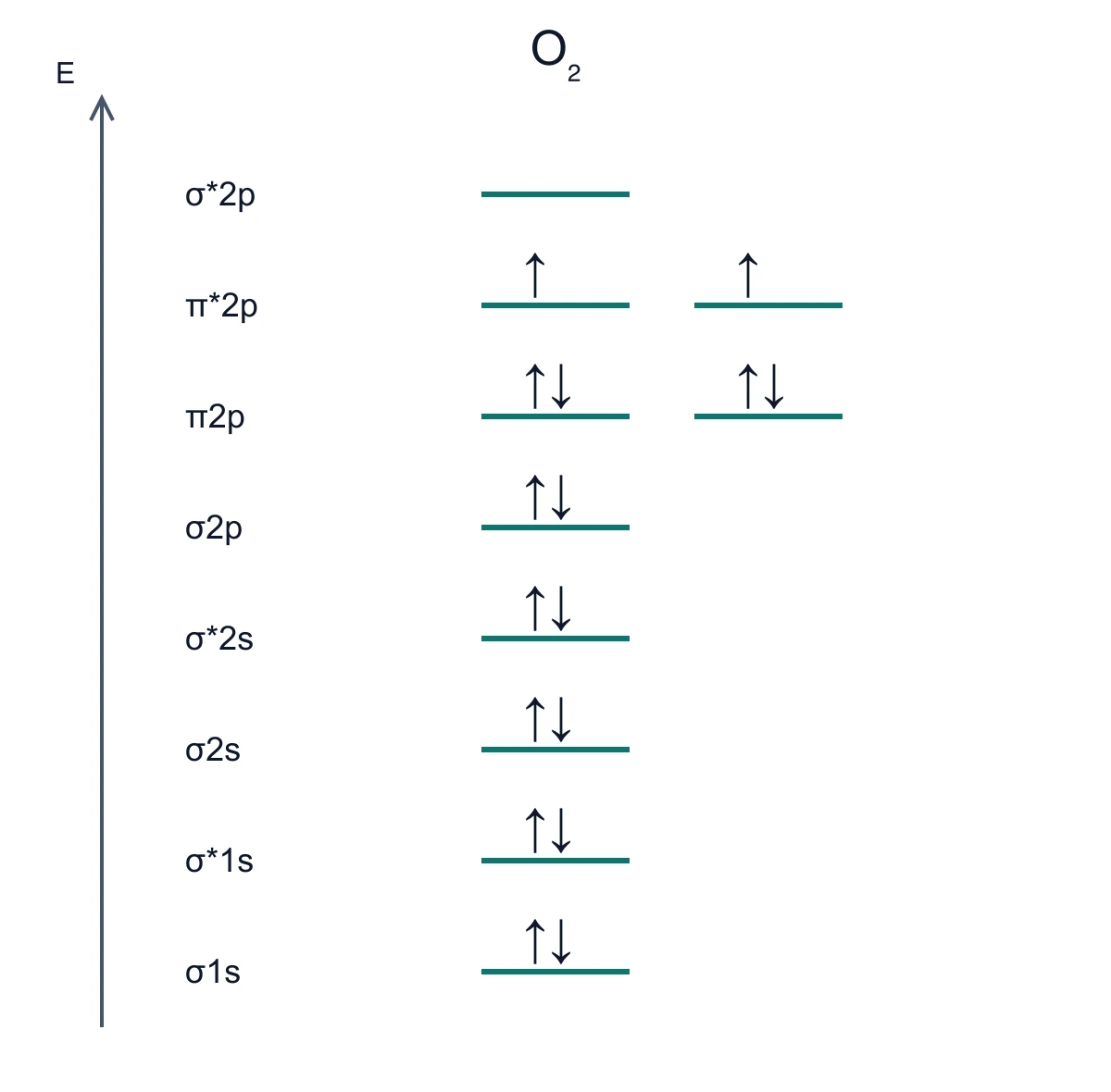 Molecular Orbital Diagram Generator
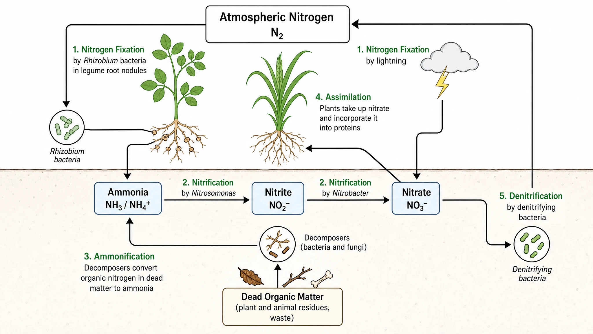 Nitrogen Cycle Diagram Generator
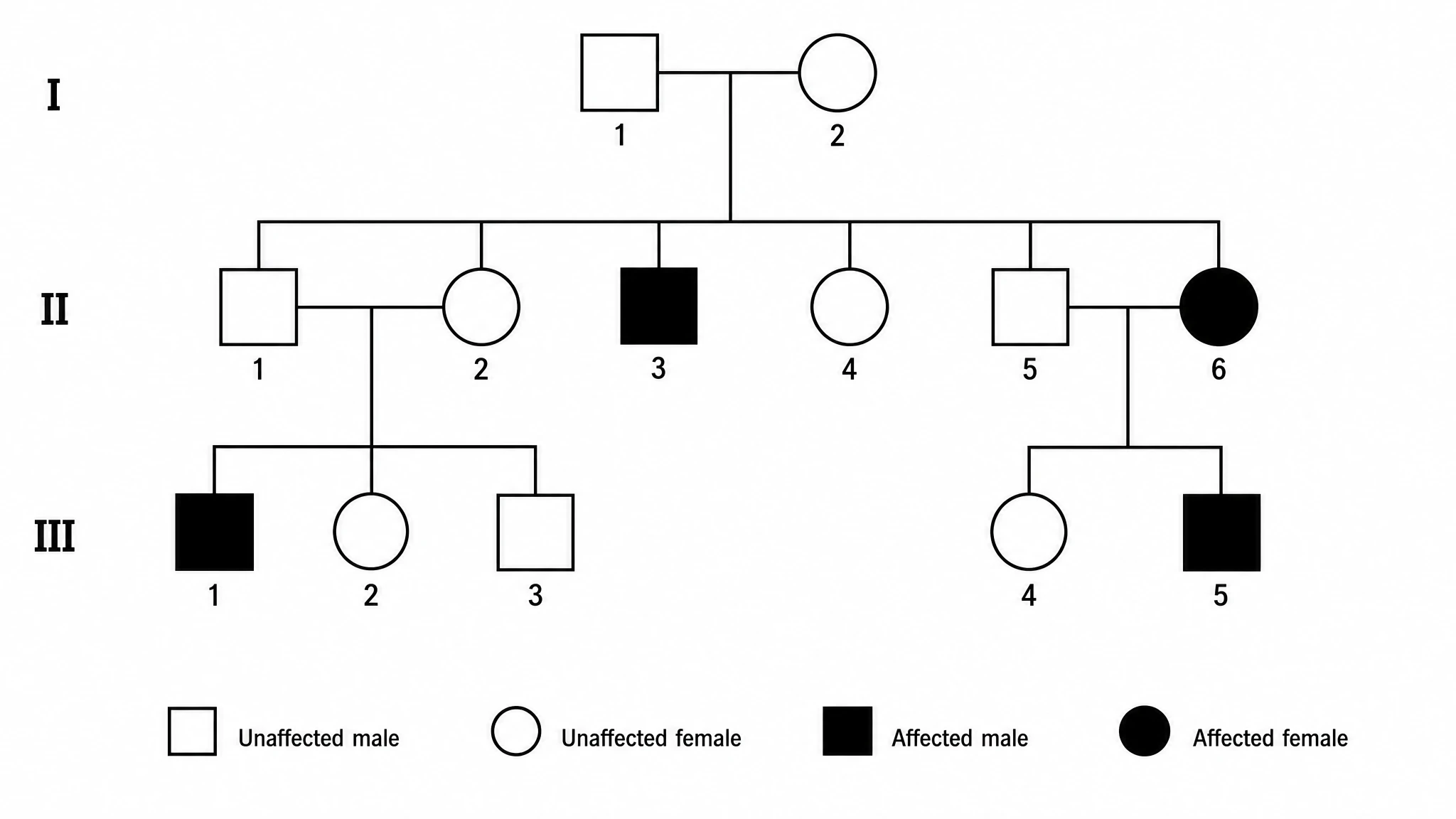 Pedigree Chart Maker
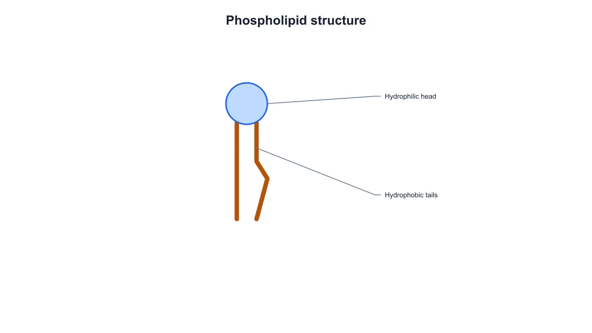 Phospholipid Diagram Generator
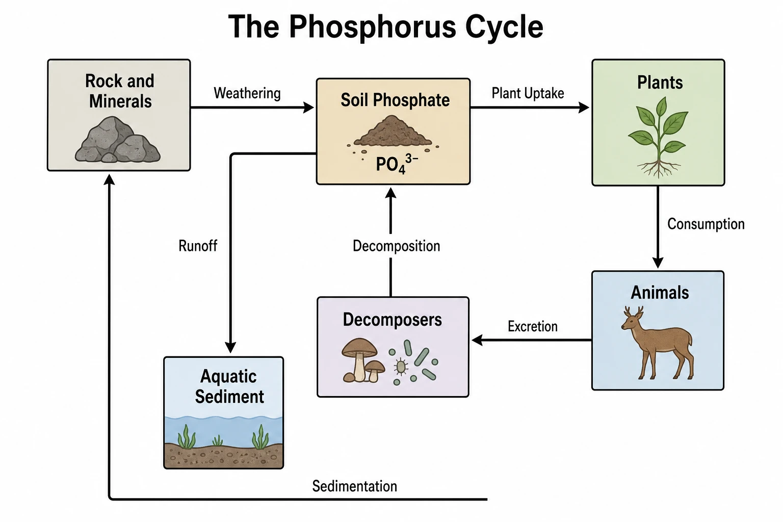 Phosphorus Cycle Diagram Generator
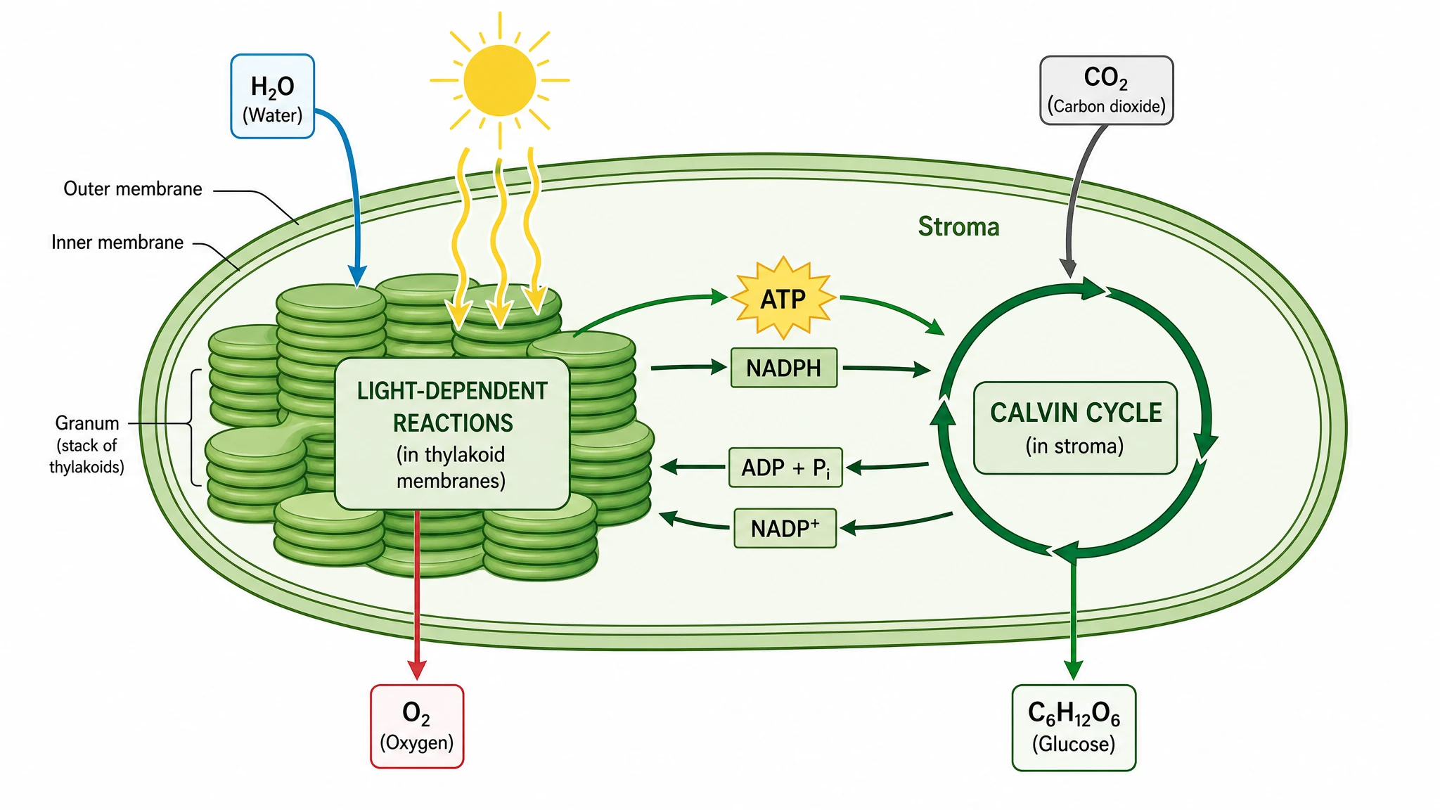 Photosynthesis Diagram Generator
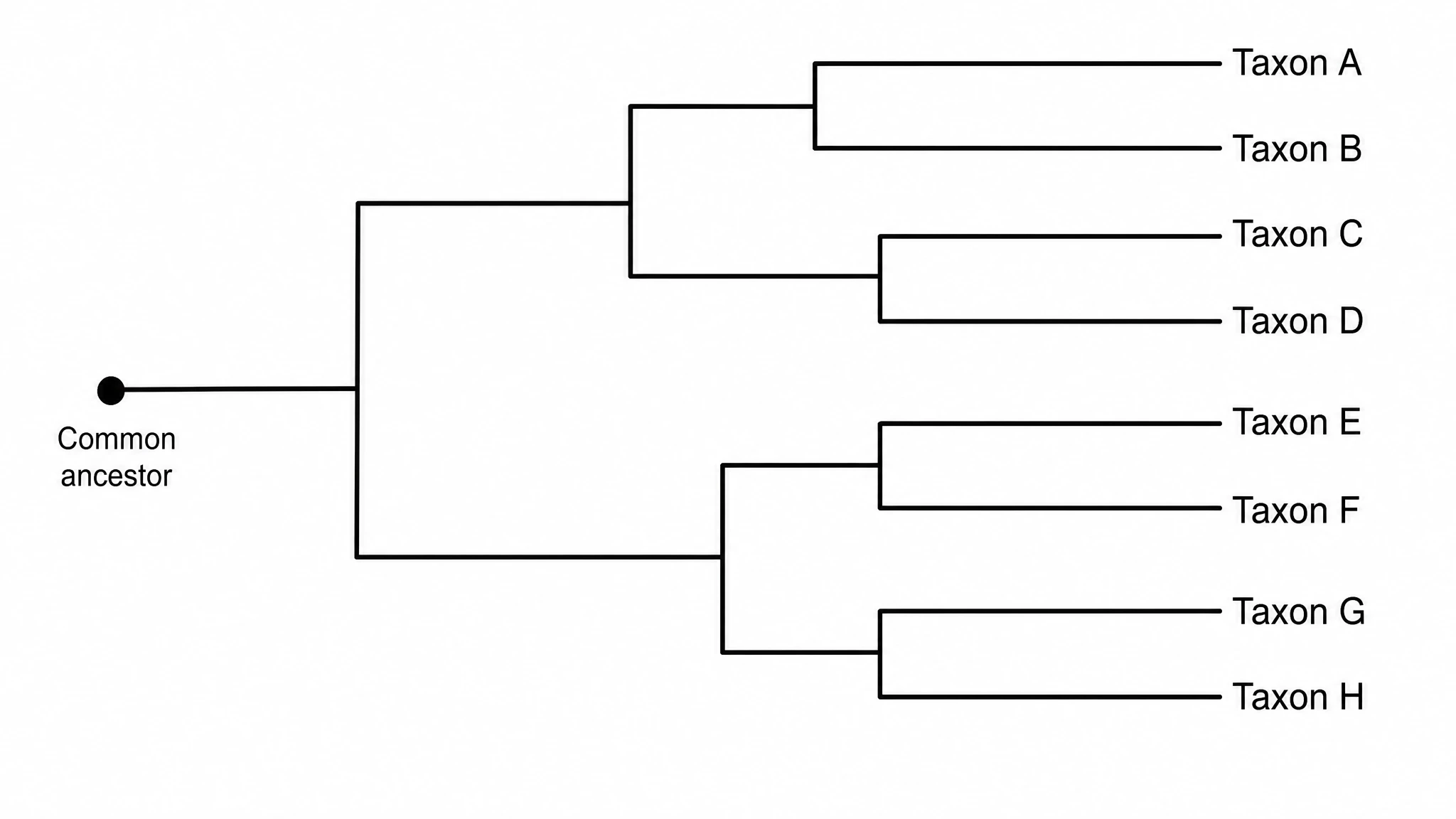 Phylogenetic Tree Maker
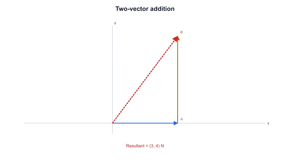 Physics Vector Diagram Maker
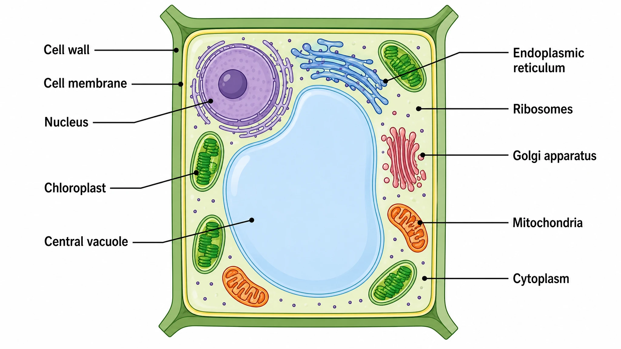 Plant Cell Diagram Generator
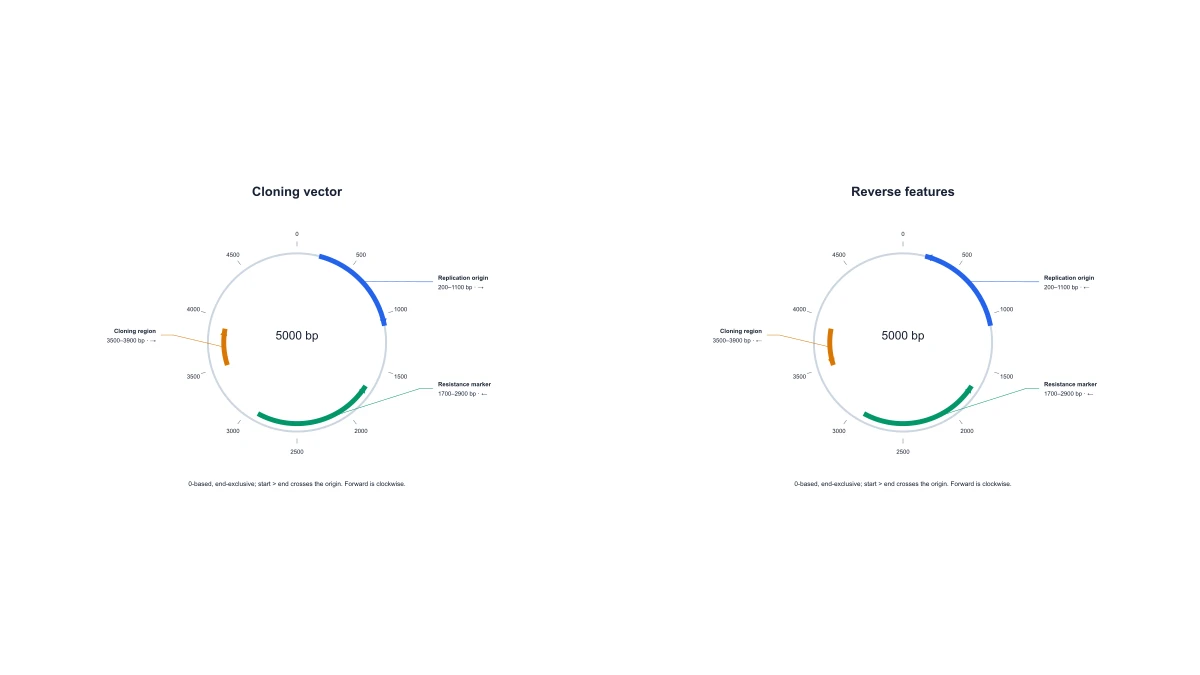 Plasmid Map Maker
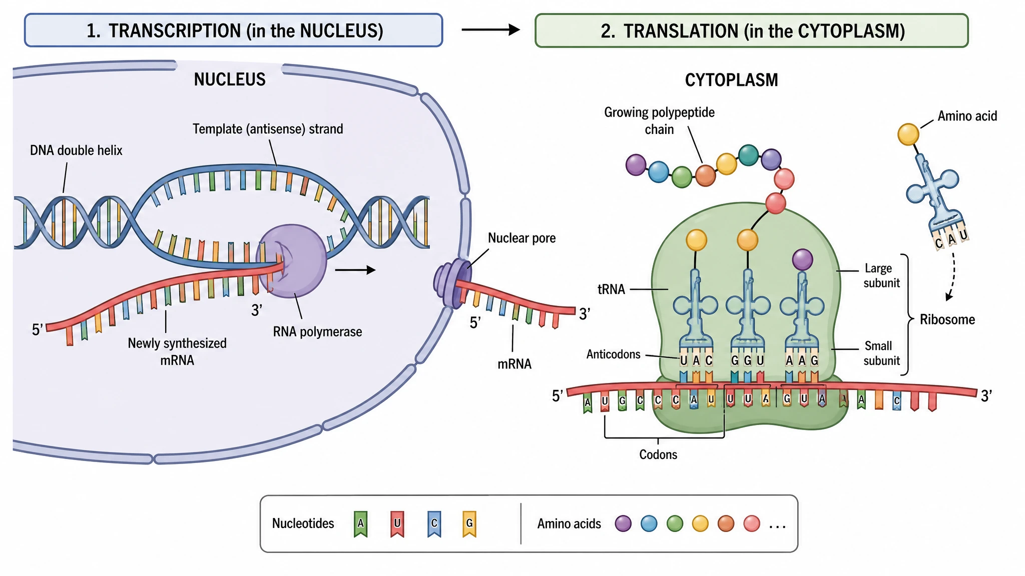 Protein Synthesis Diagram Generator
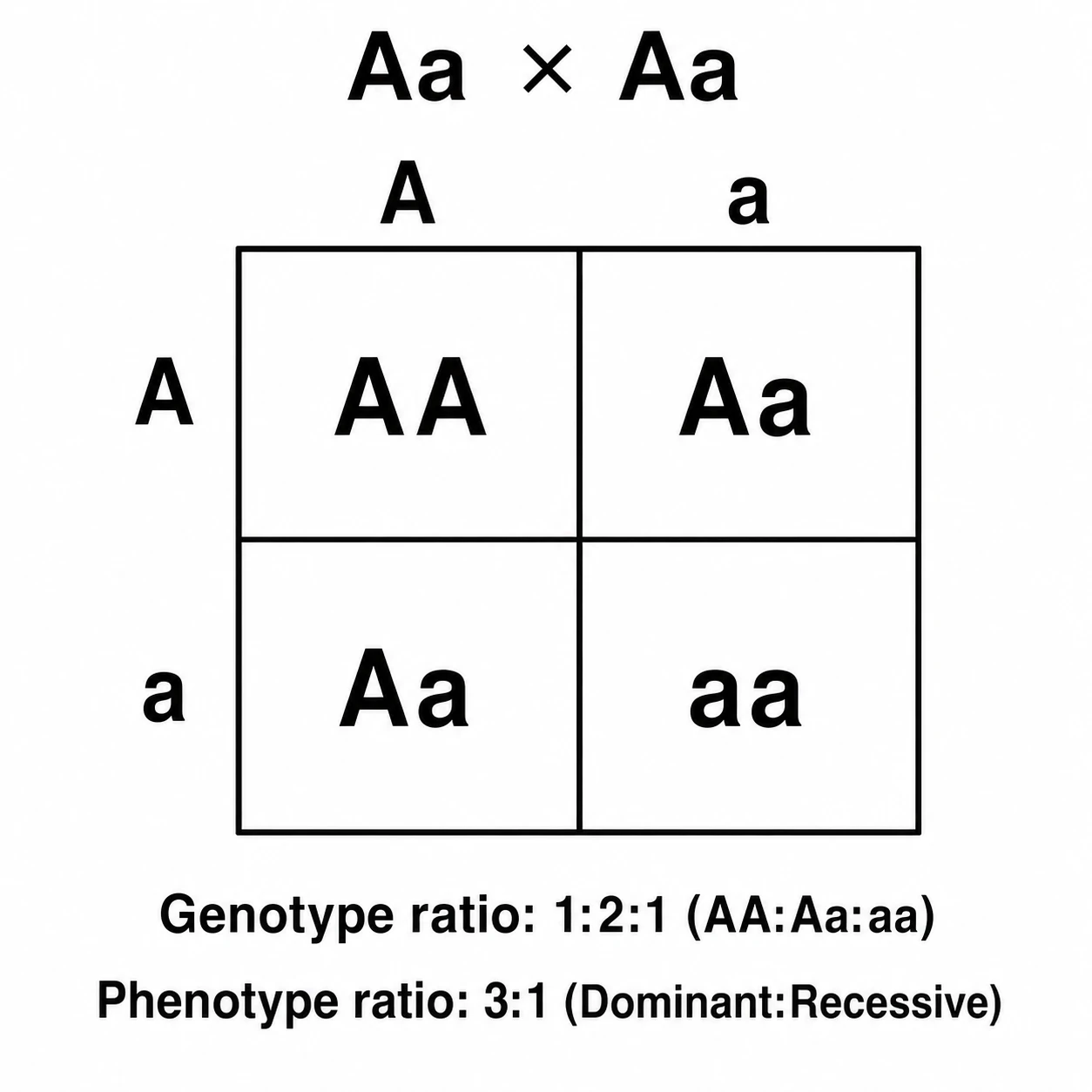 Punnett Square Maker
 Ray Diagram Maker
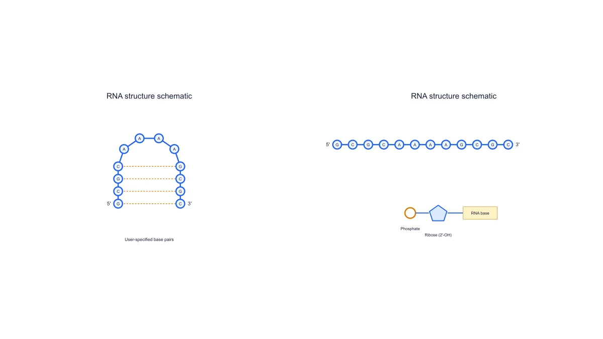 RNA Structure Diagram Generator
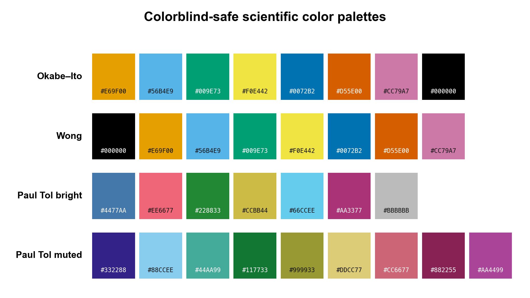 Scientific Color Palette Generator
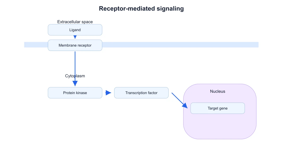 Signaling Pathway Diagram Generator
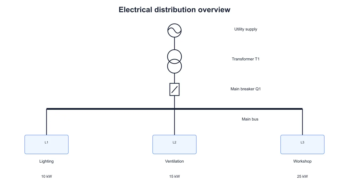 Single Line Diagram Generator
 T-Cell Activation Diagram Generator
 Water Cycle Diagram Generator
 Western Blot Diagram Generator
Statistical charts and graphs
32 tools Bode Plot Generator
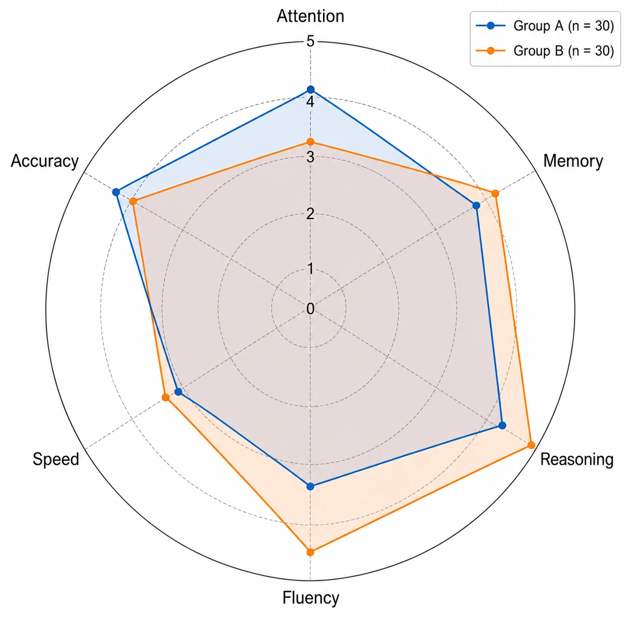 Spider Chart Maker
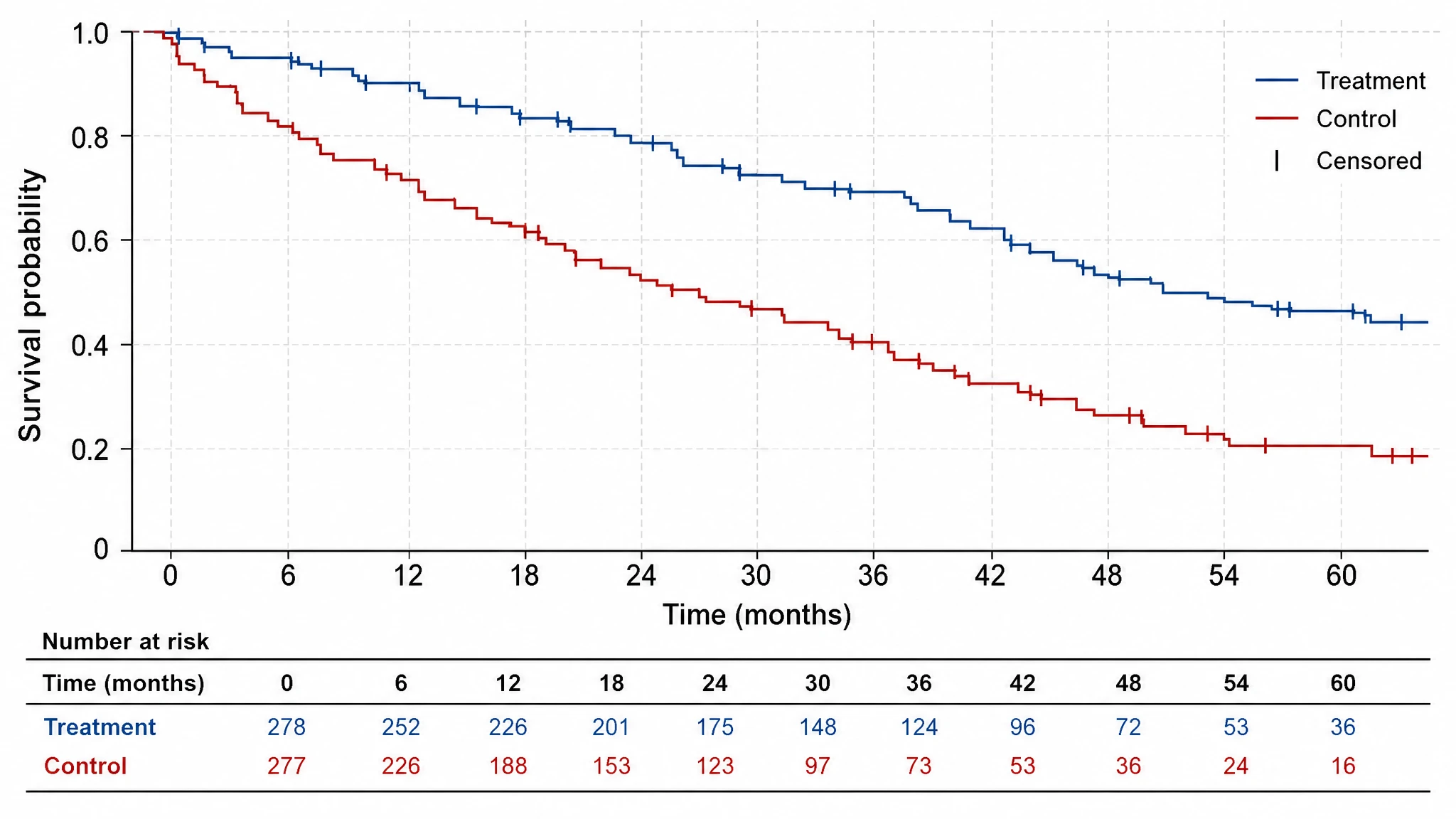 Kaplan-Meier Survival Curve
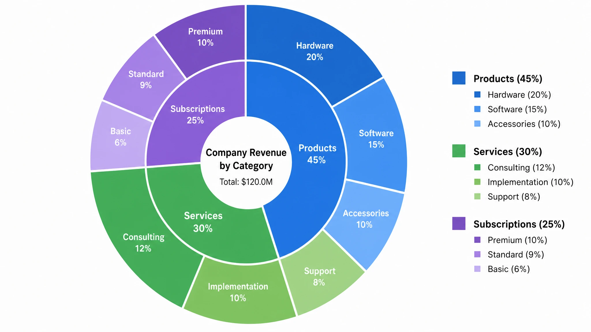 Multi-Layer Pie Chart Maker
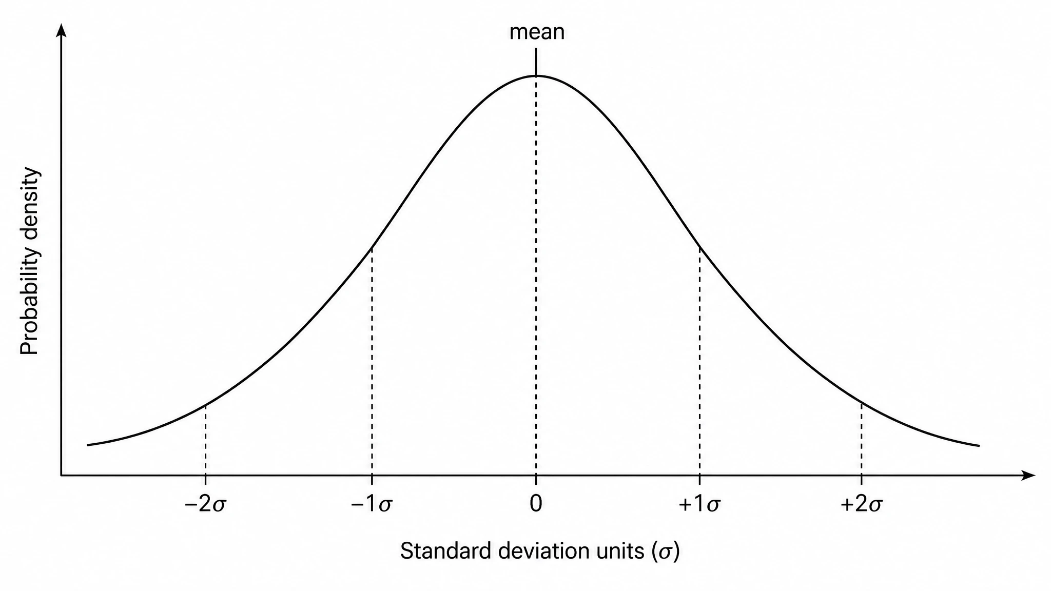 Bell Curve Generator
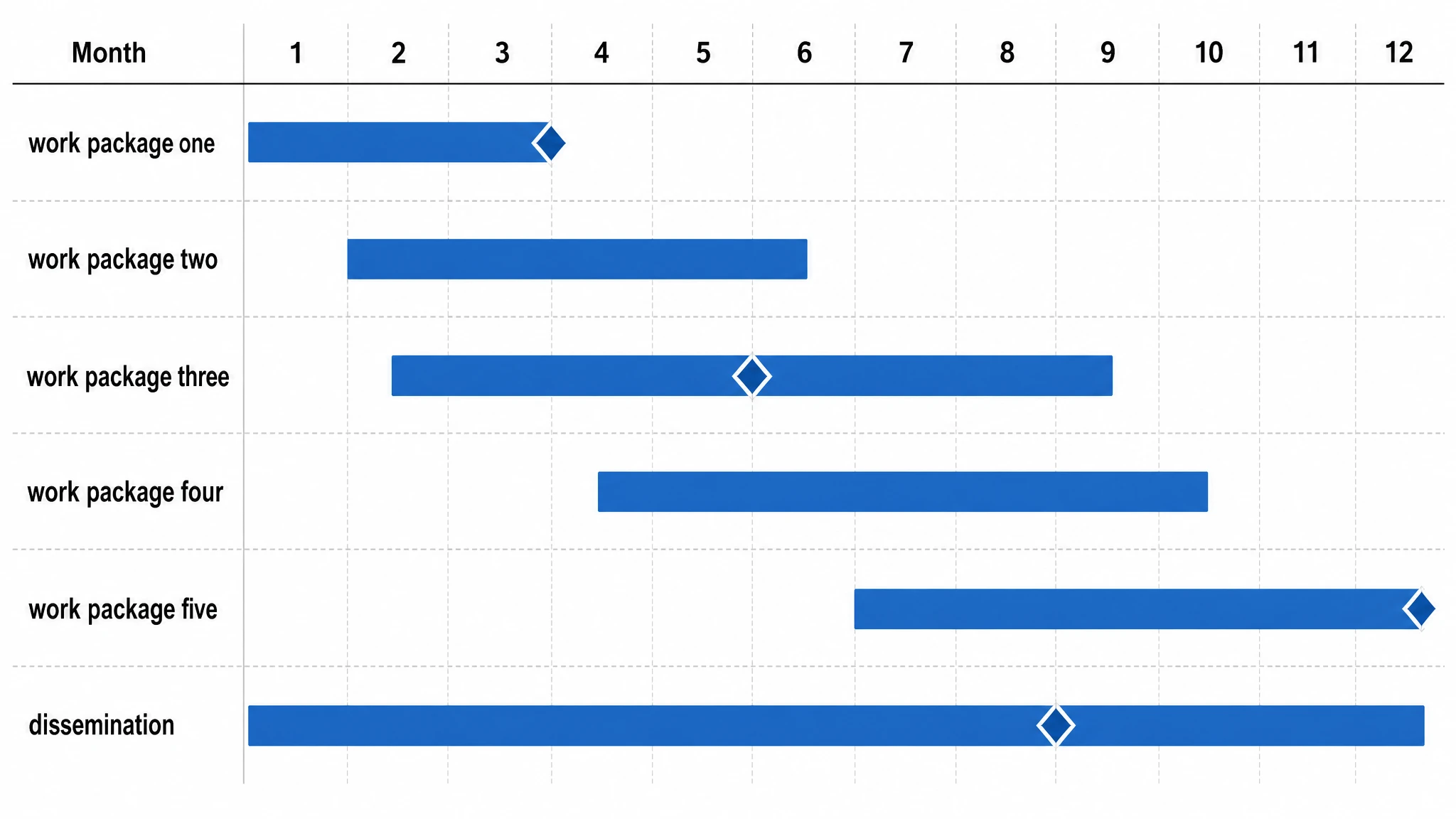 Gantt Chart Generator
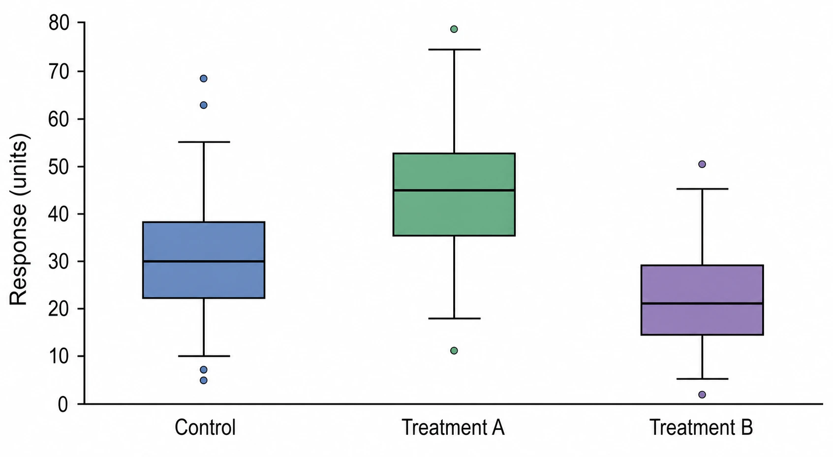 Box Plot Generator
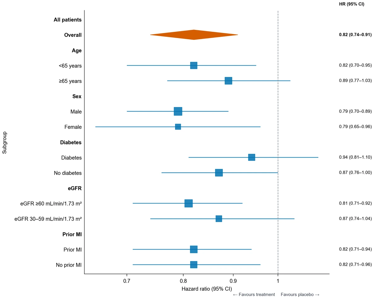 Forest Plot Generator
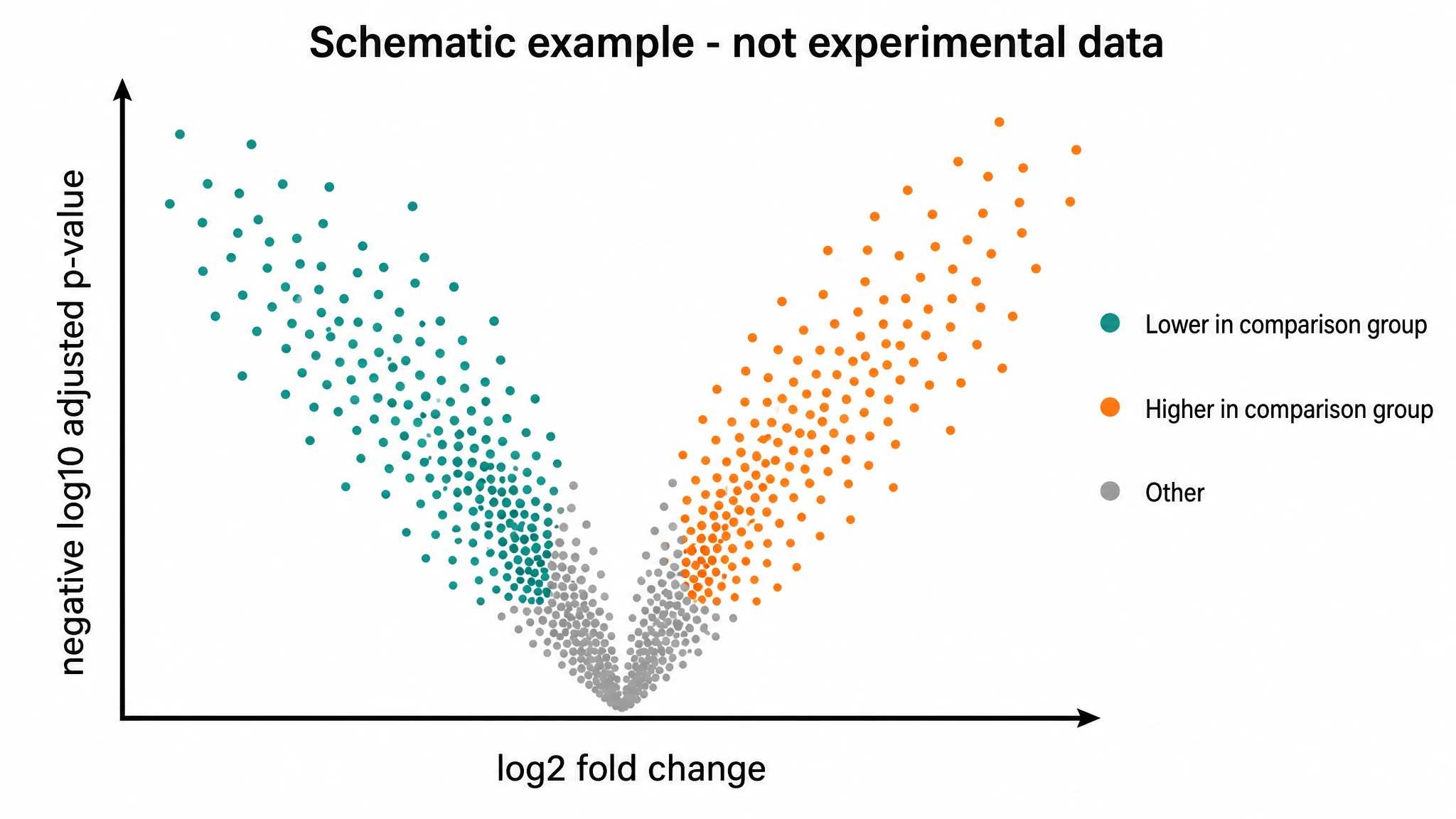 Volcano Plot Generator
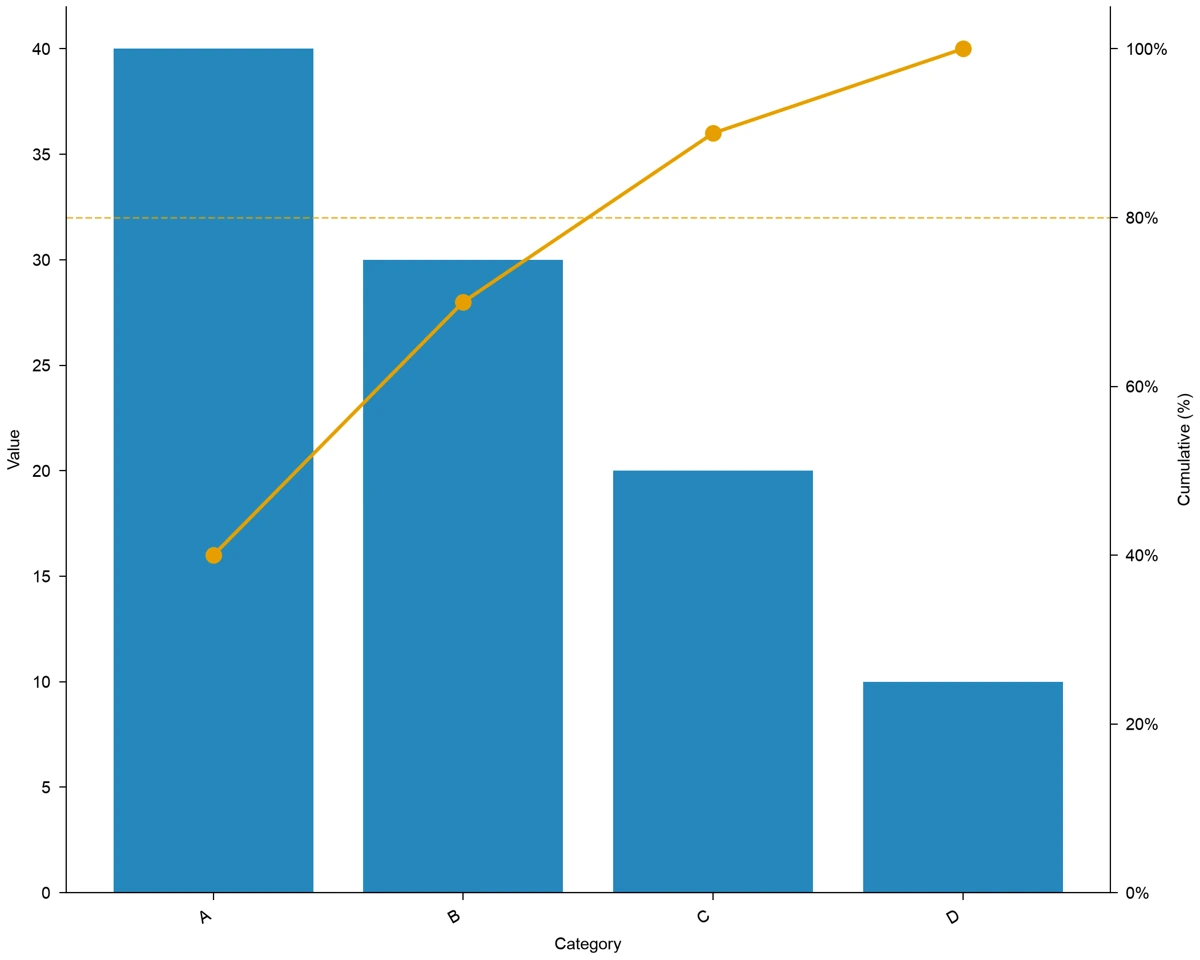 Pareto Chart Maker
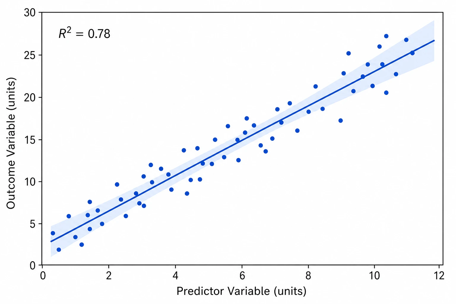 Scatter Plot Maker
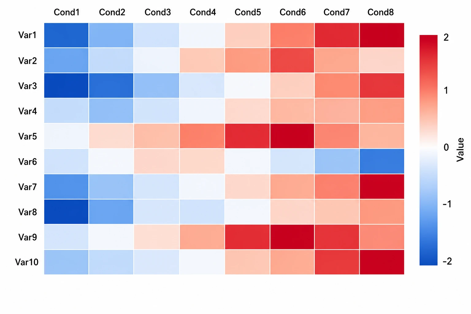 Heatmap Generator
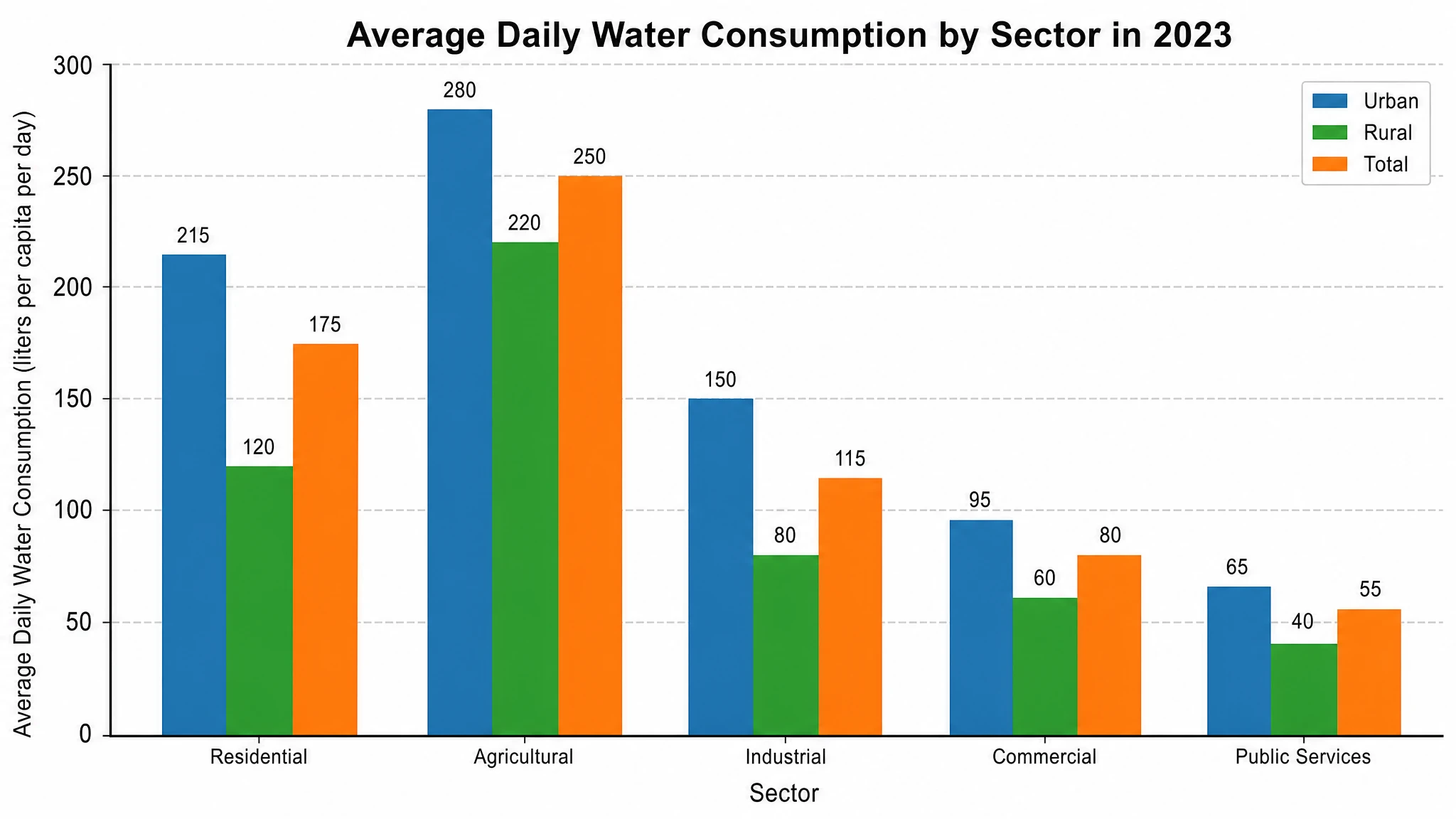 AI Chart Generator
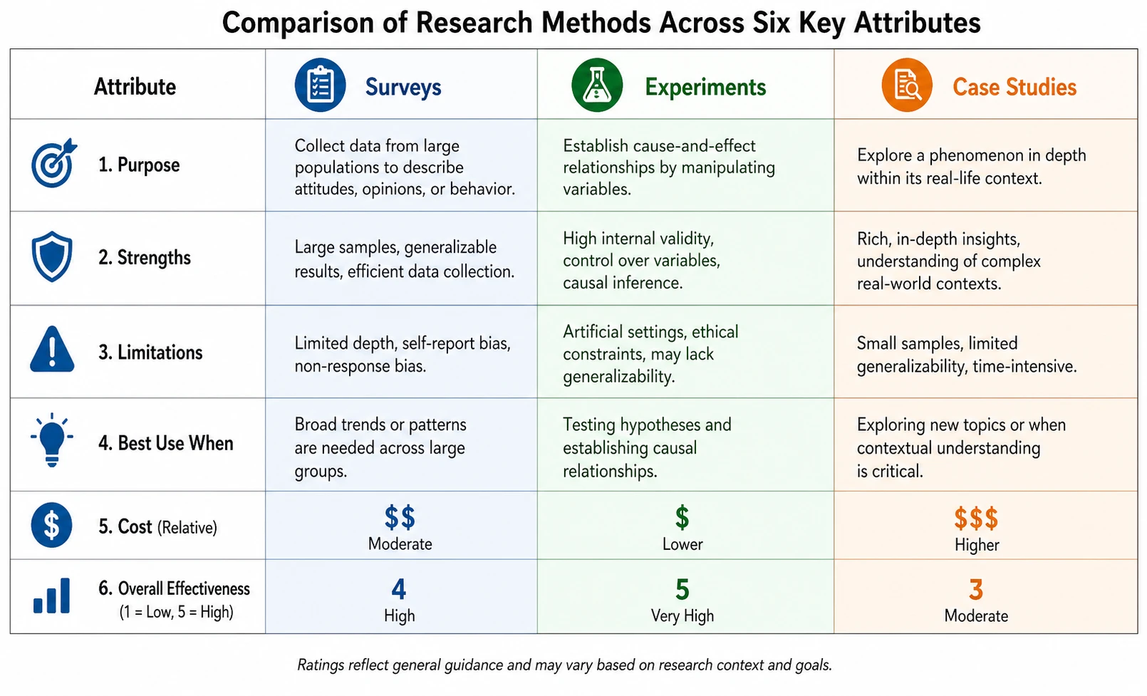 Comparison Chart Maker
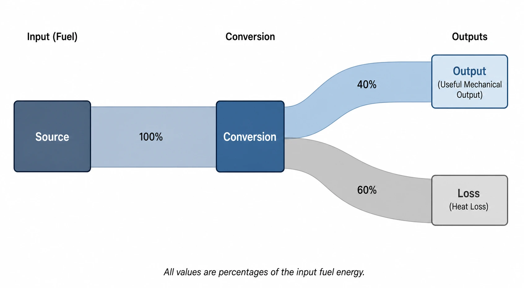 Sankey Diagram Generator
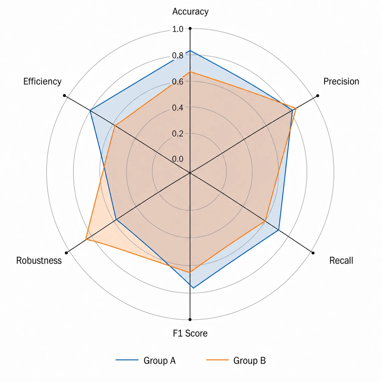 Radar Chart Generator
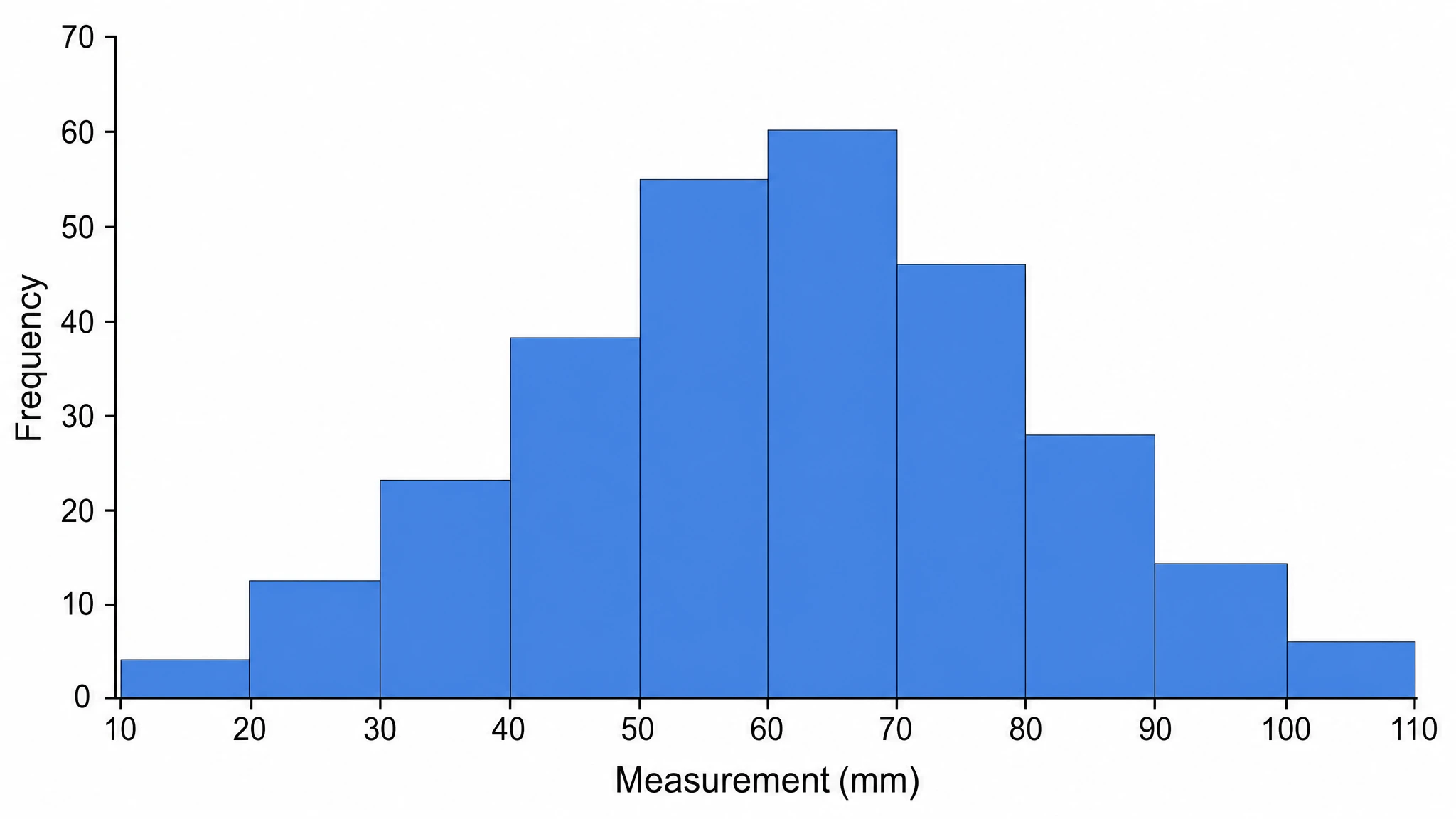 Histogram Maker
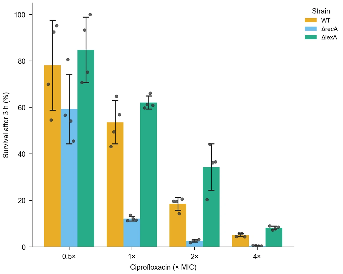 Bar Chart Generator
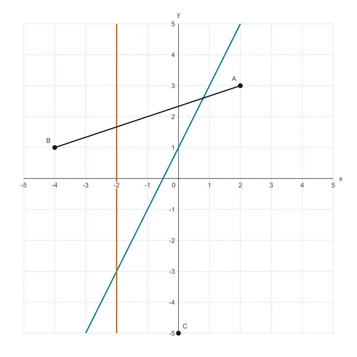 Coordinate Plane Generator
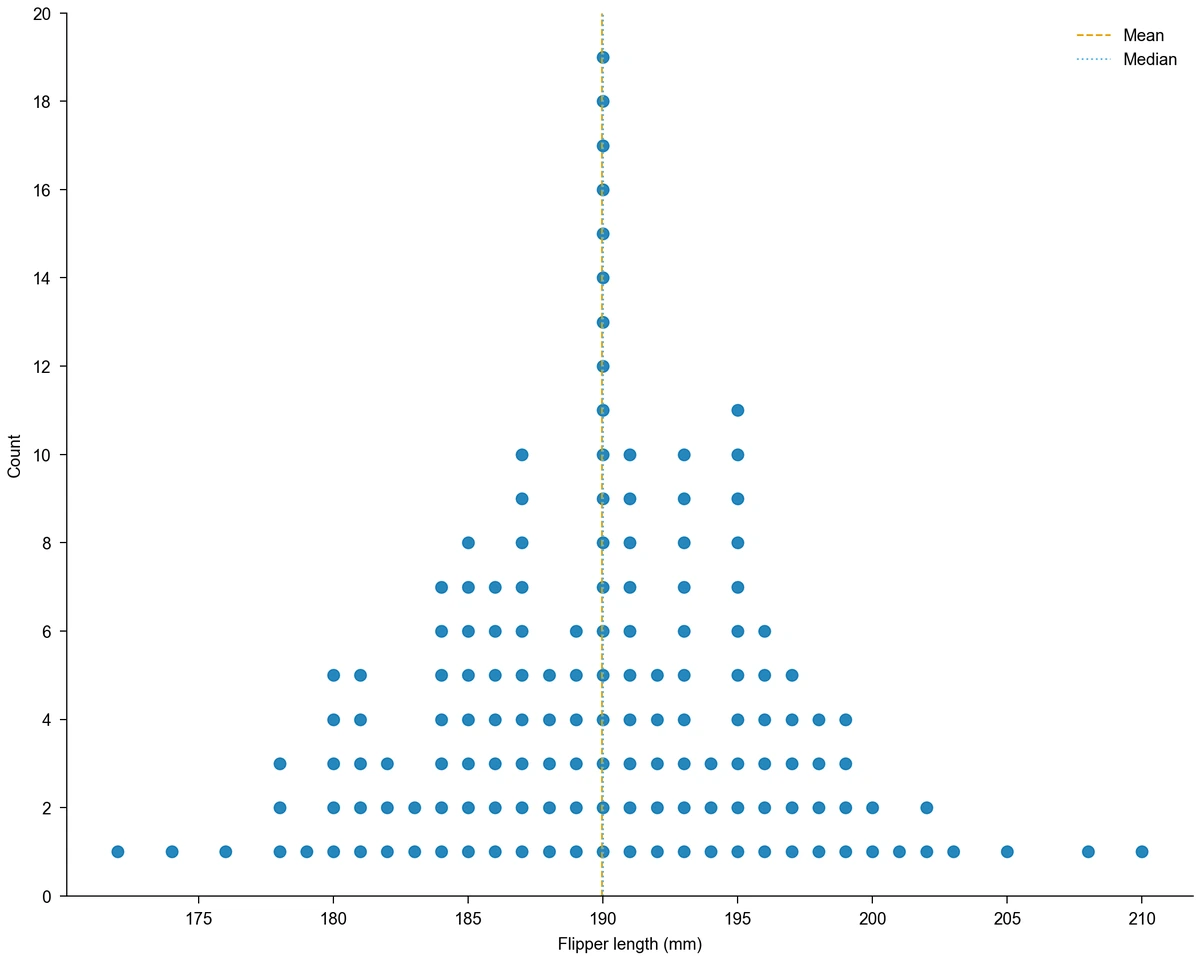 Dot Plot CreatorWater Heating Curve
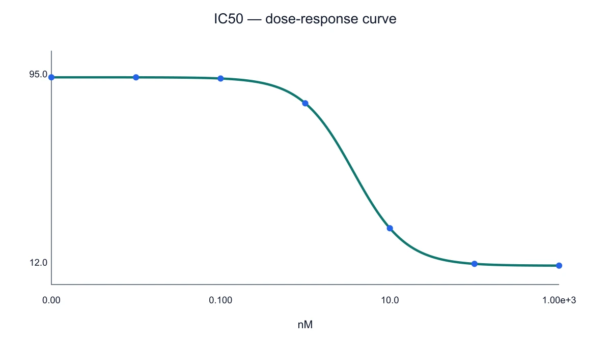 IC50 Calculator & Dose-Response Curves
 Image DPI Calculator
 Transverse Wave Diagram Generator
 Line Chart Generator
 MA Plot
 Number Line Generator
 Figure Checker
 Scientific Graph Maker
 Supply and Demand Graph Maker
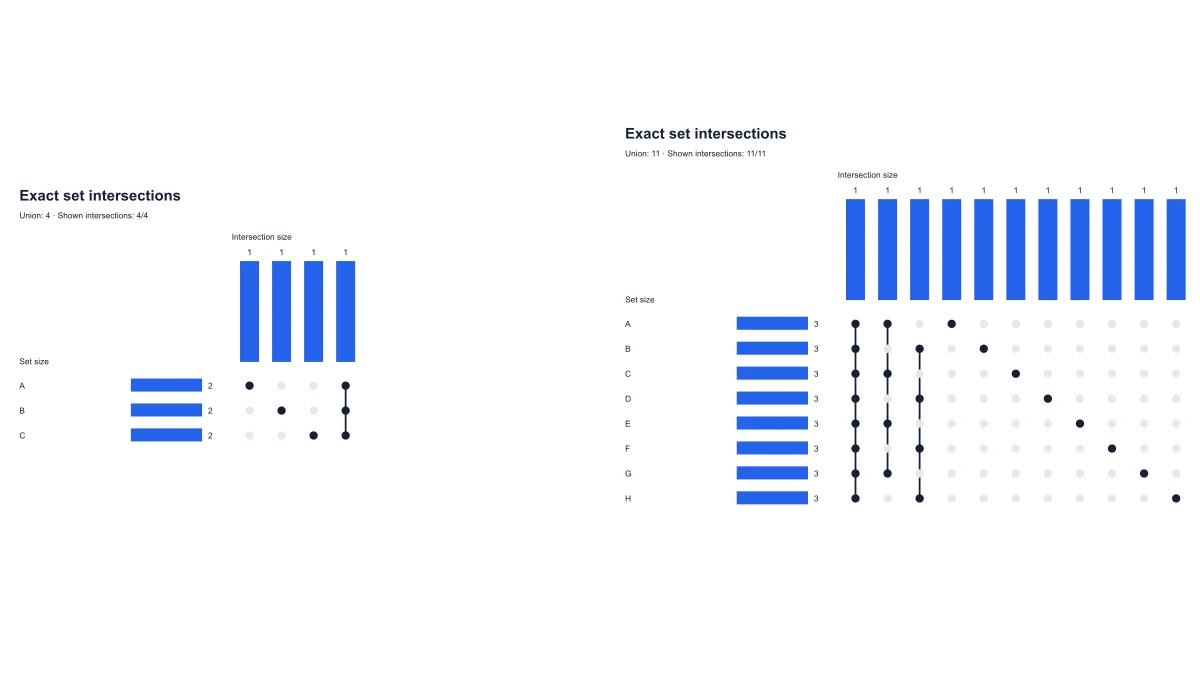 UpSet Plot Generator
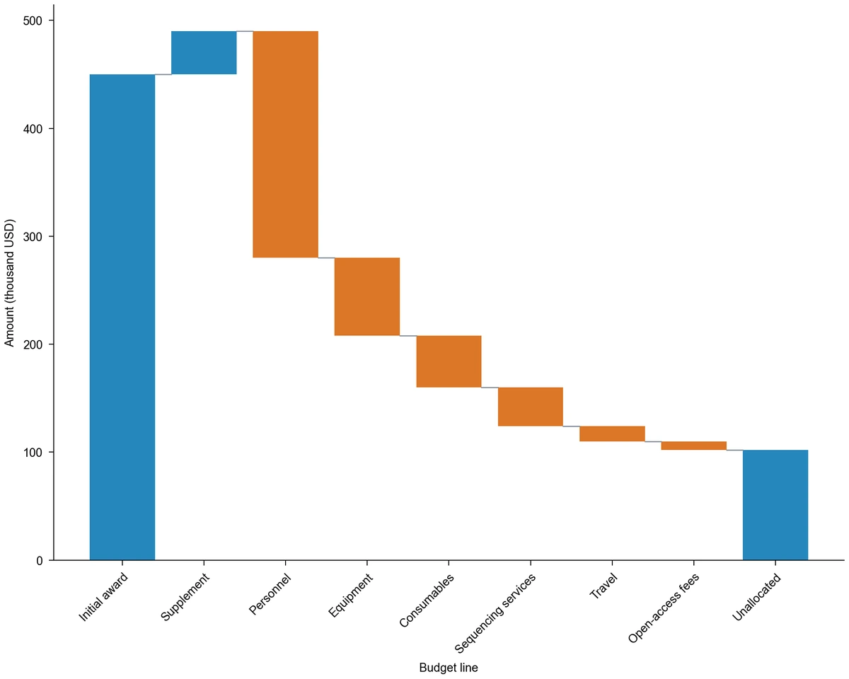 Waterfall Chart Maker
Flowcharts, frameworks and structure diagrams
33 tools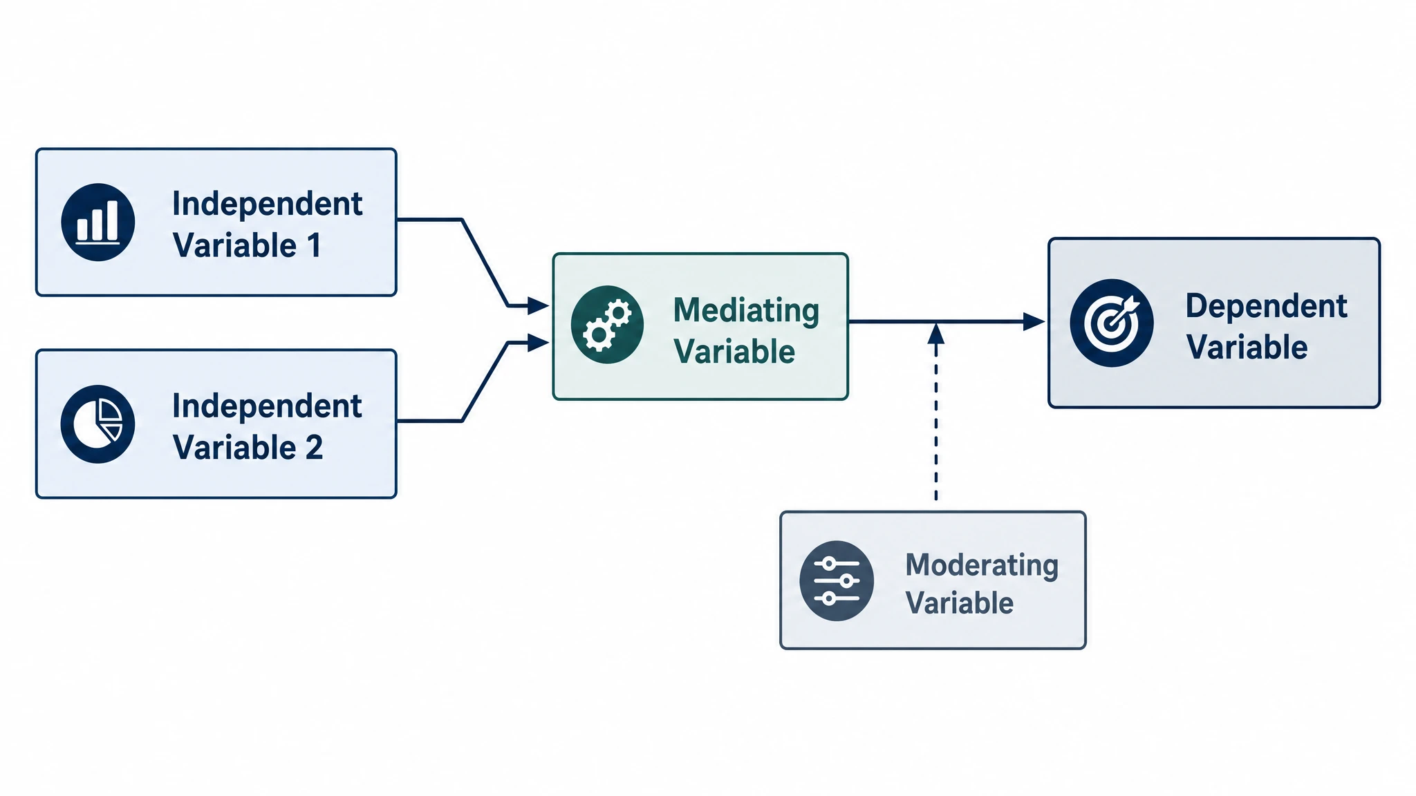 Conceptual Framework Generator
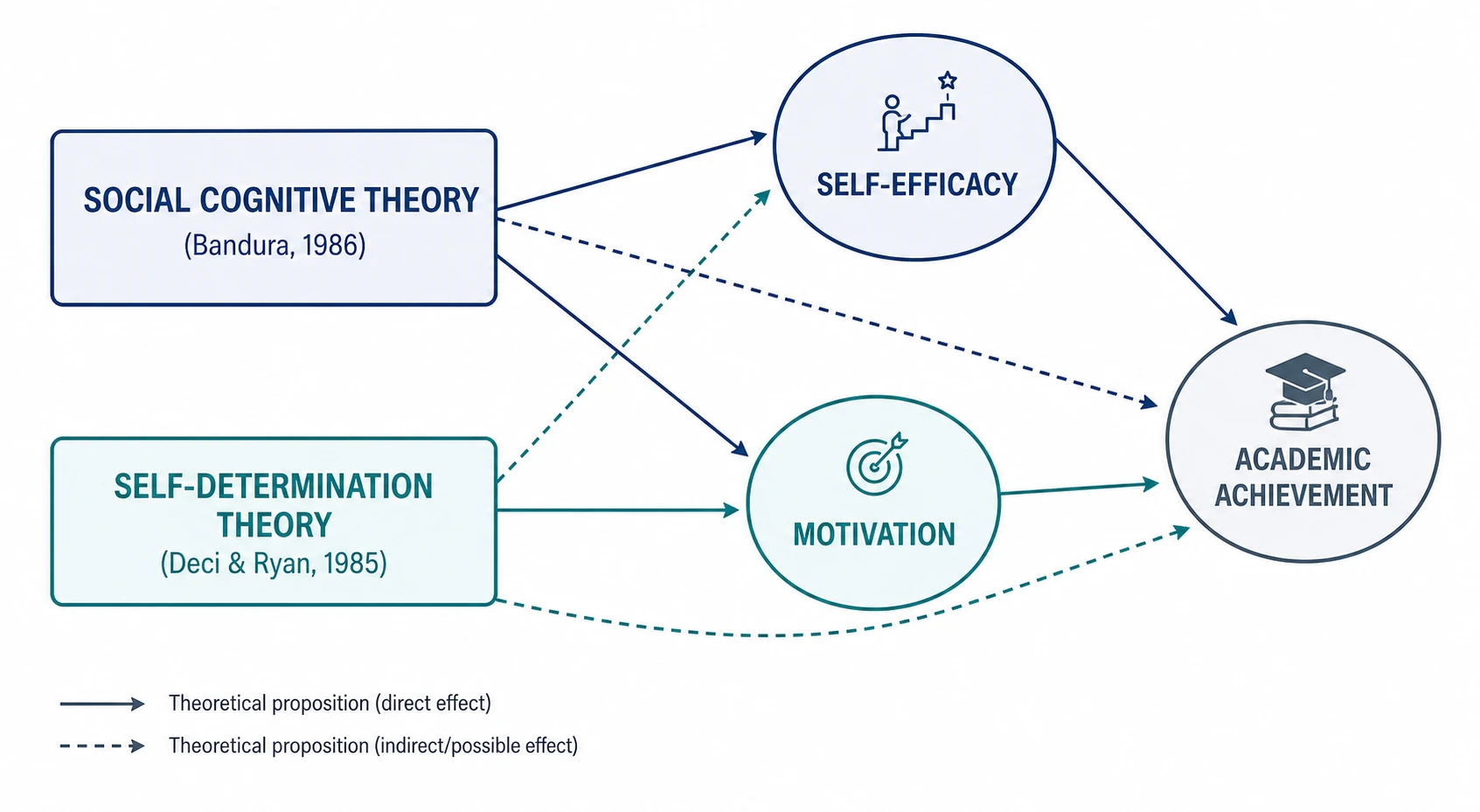 Theoretical Framework Generator
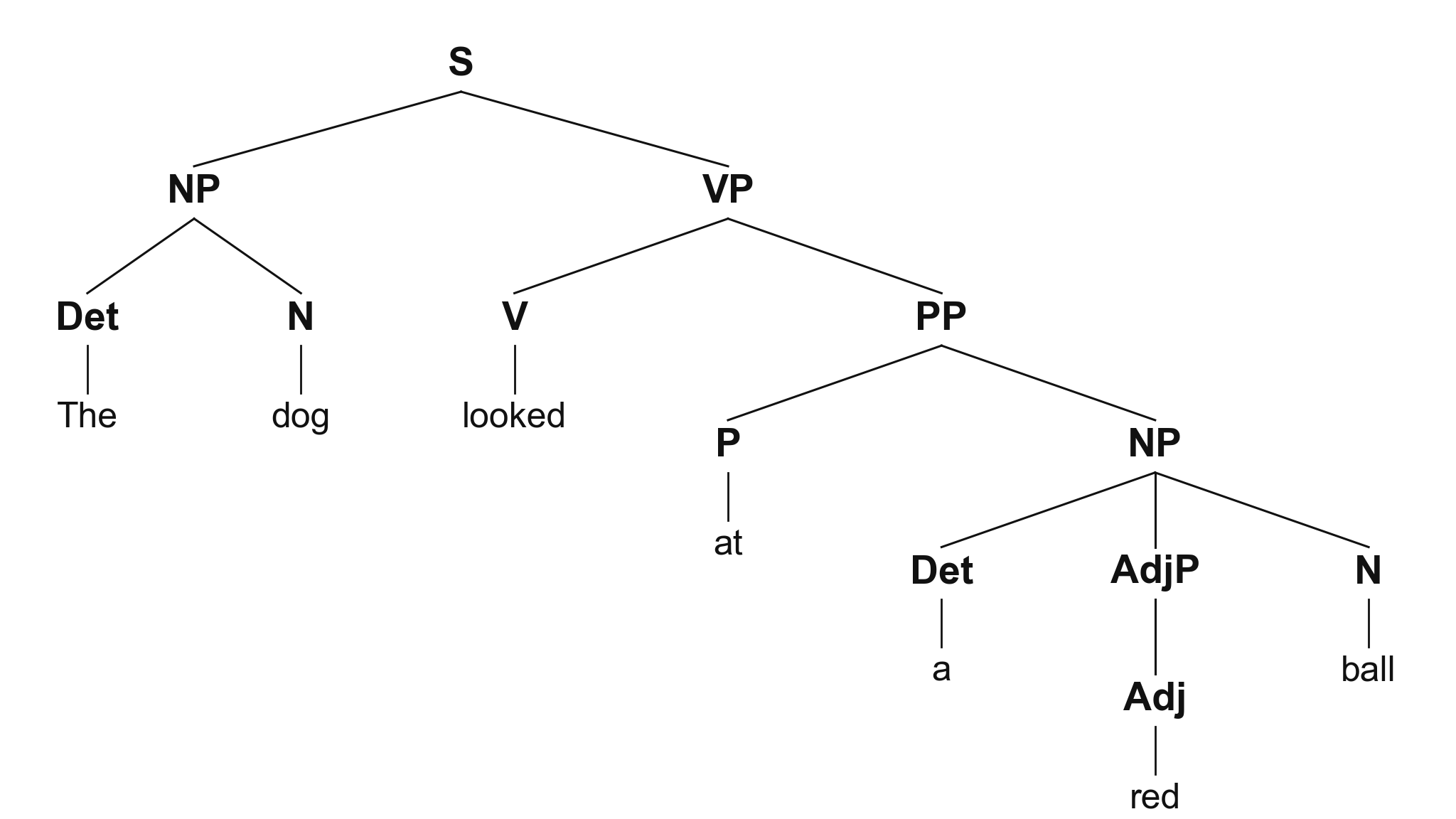 Syntactic Tree Generator
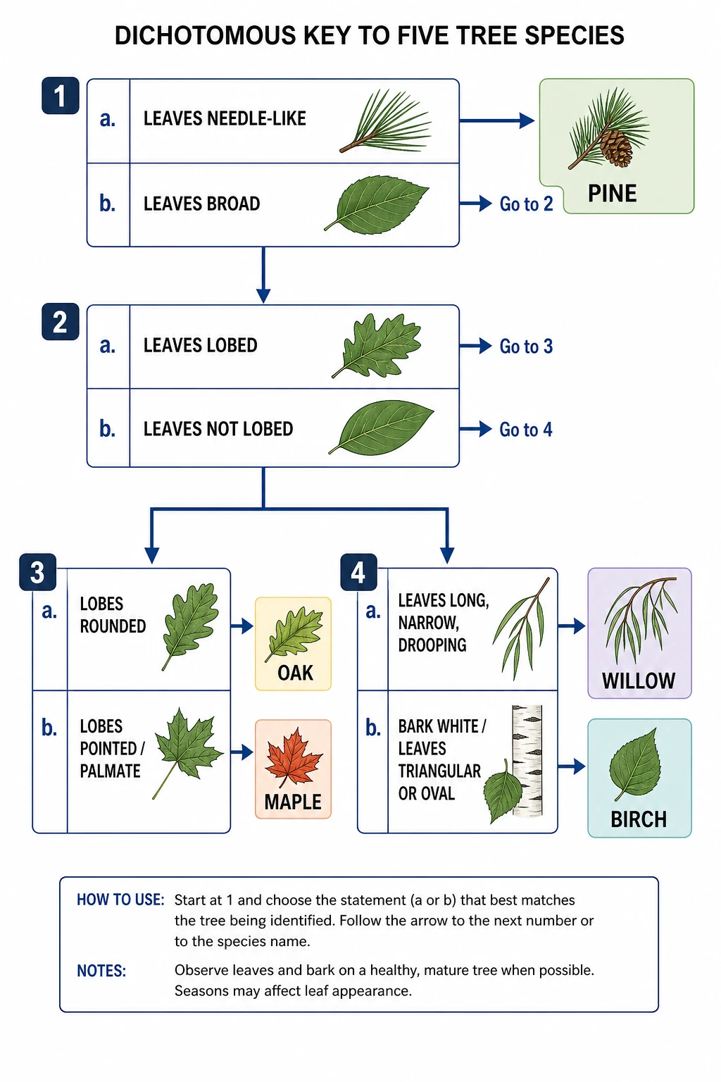 Dichotomous Key Maker
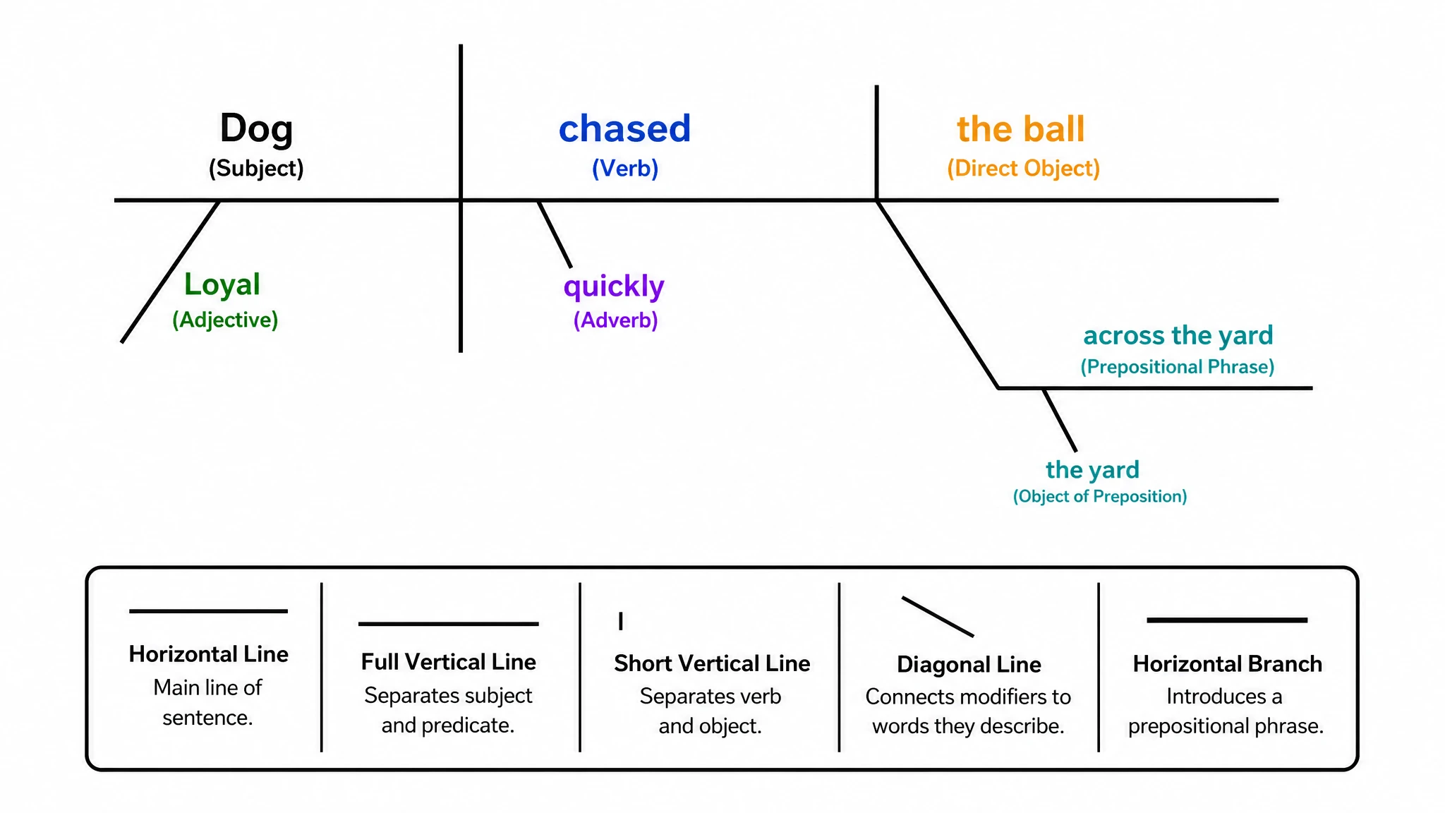 Sentence Diagram Generator
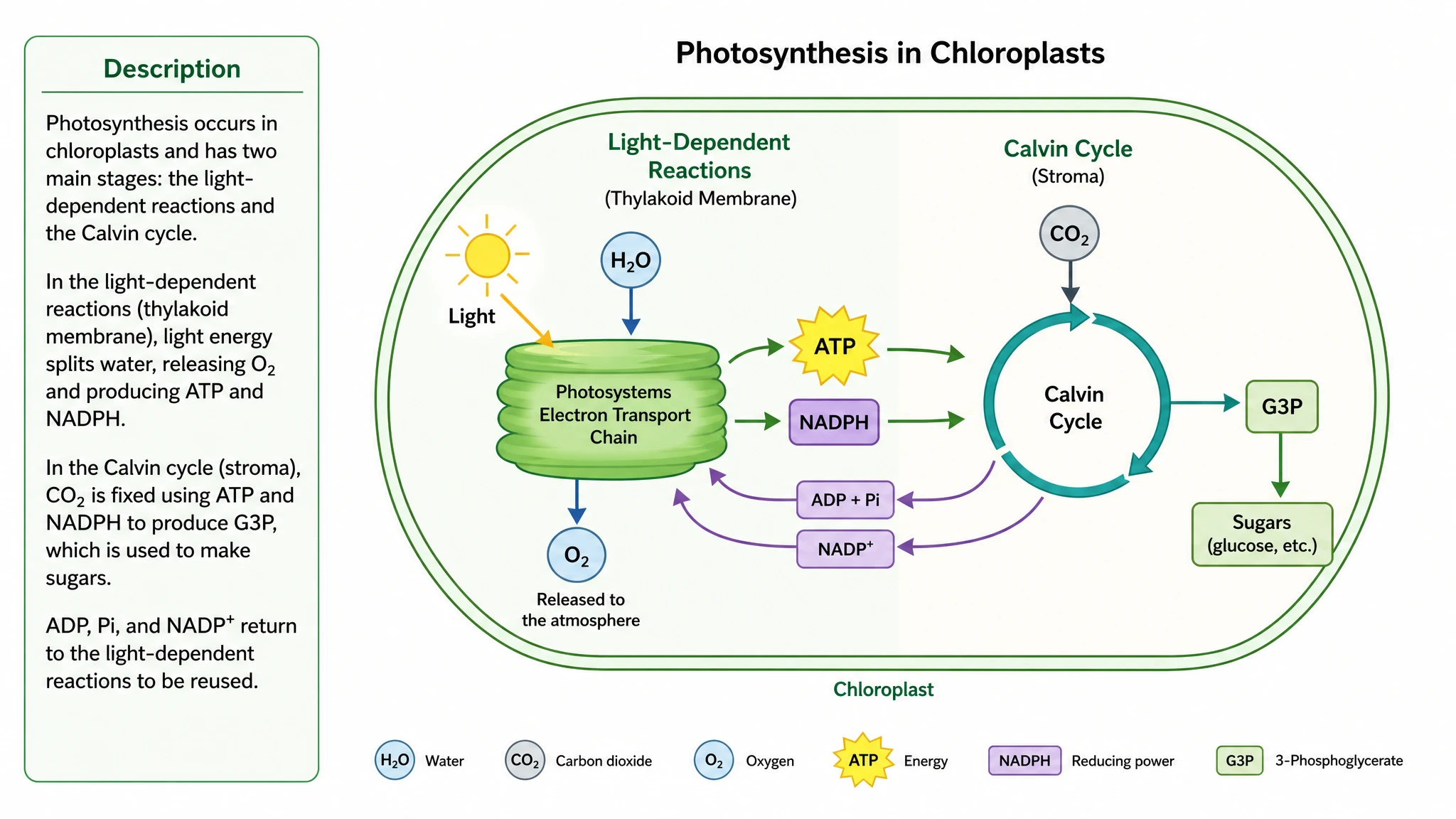 Text to Diagram Generator
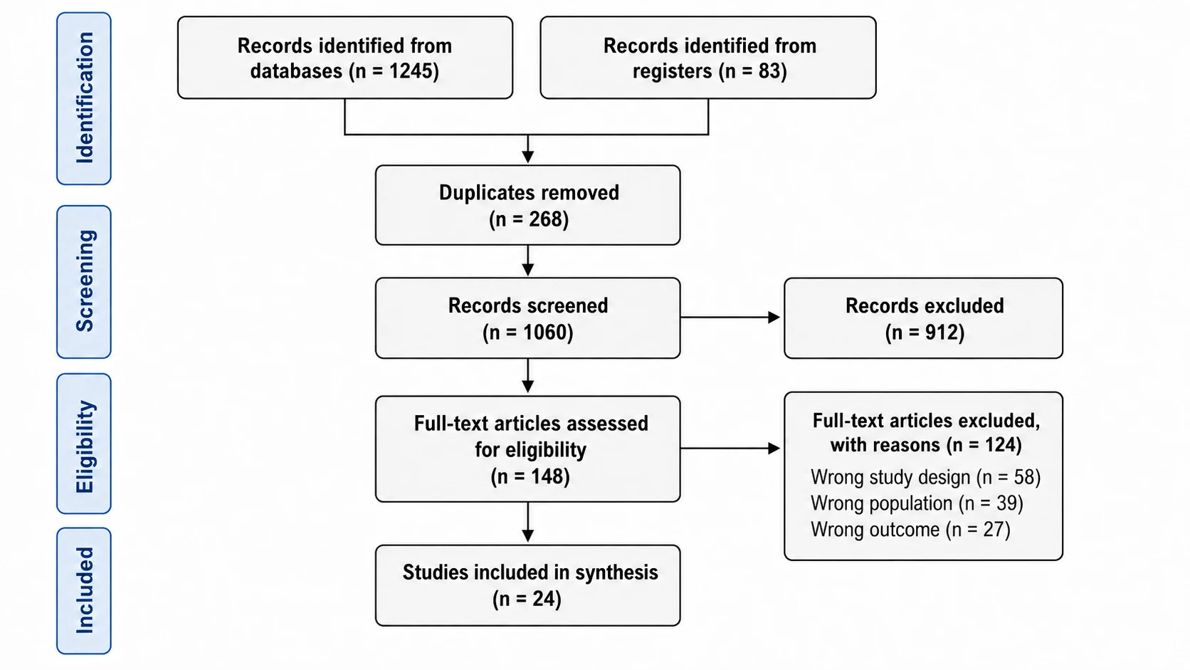 PRISMA Flow Diagram Generator
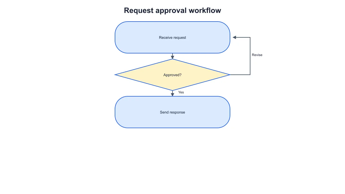 Workflow Diagram Generator
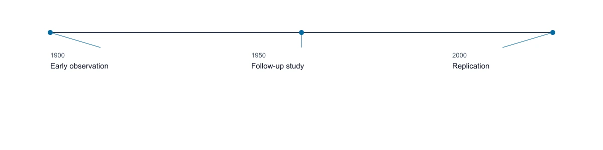 Timeline Generator
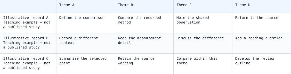 Synthesis Matrix Generator
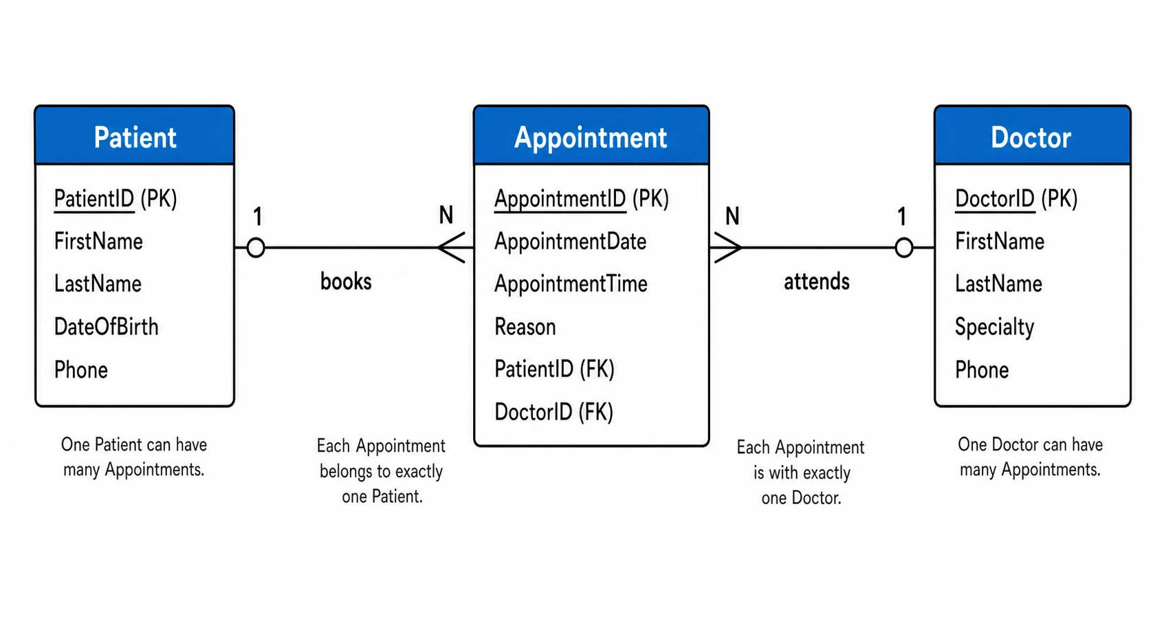 ER Diagram Generator
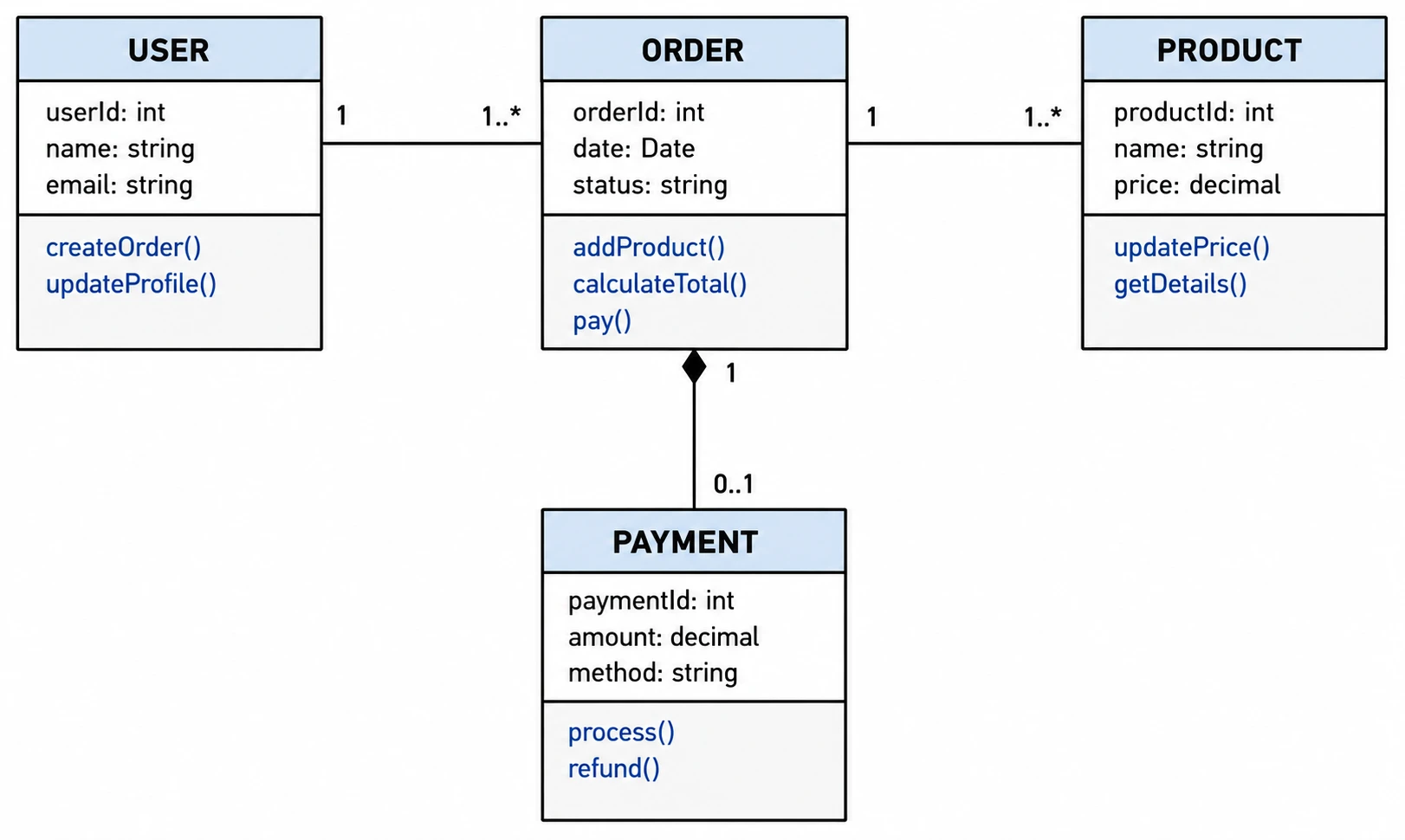 UML Diagram Generator
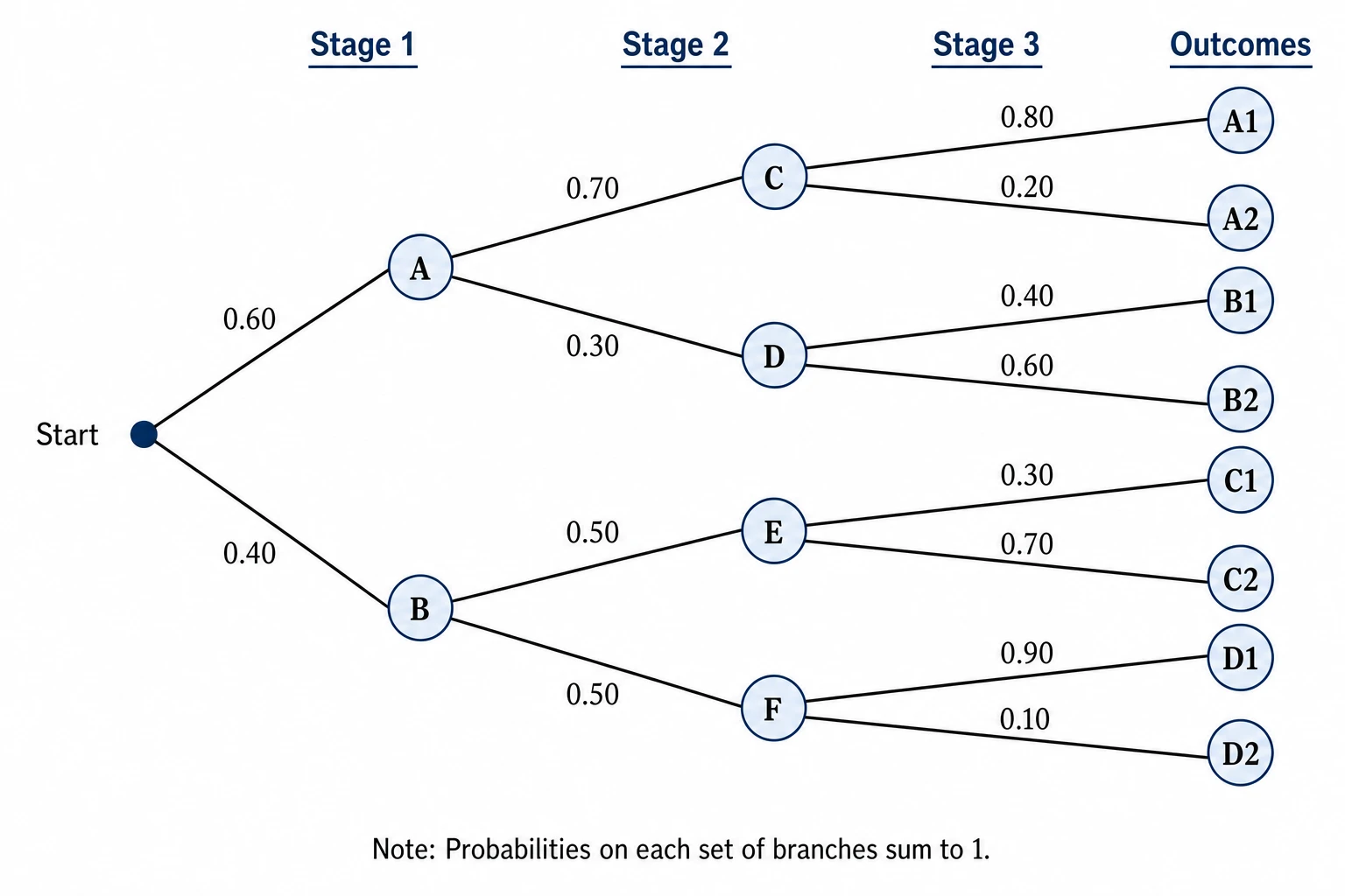 Tree Diagram Generator
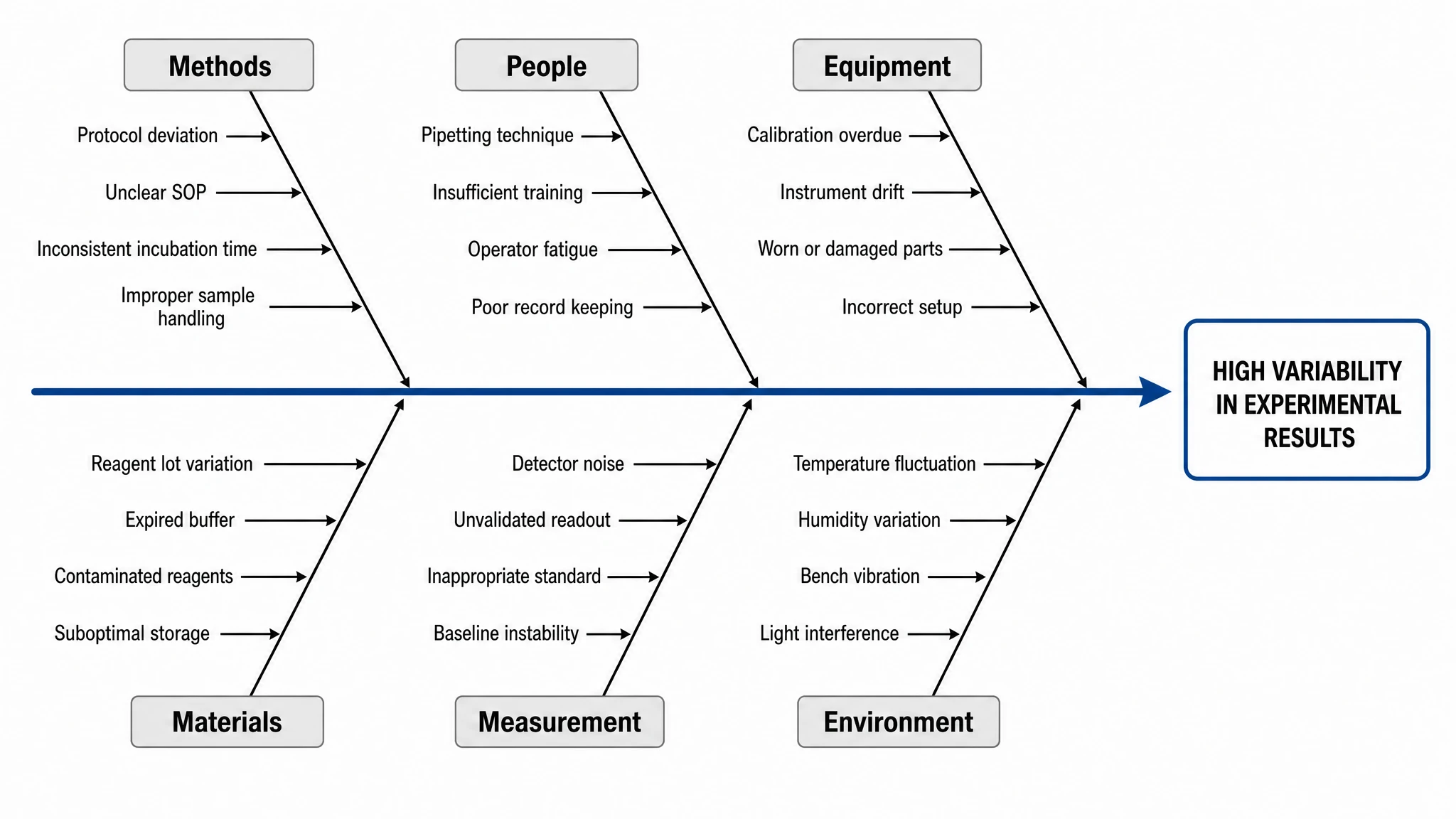 Fishbone Diagram Generator
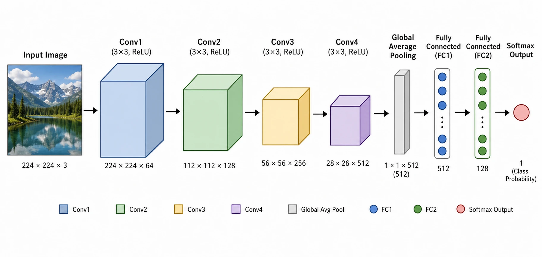 Neural Network Diagram Generator
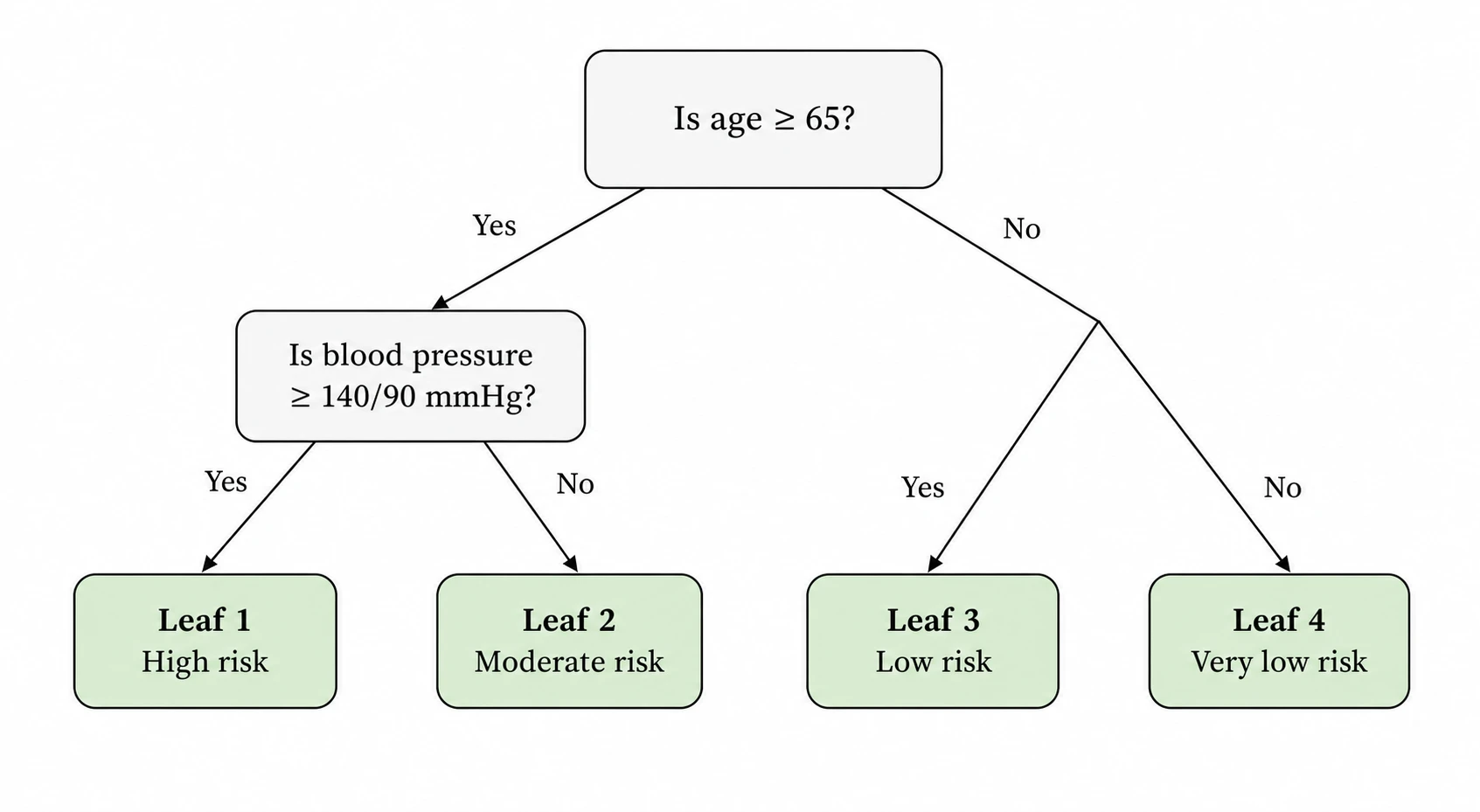 Decision Tree Generator
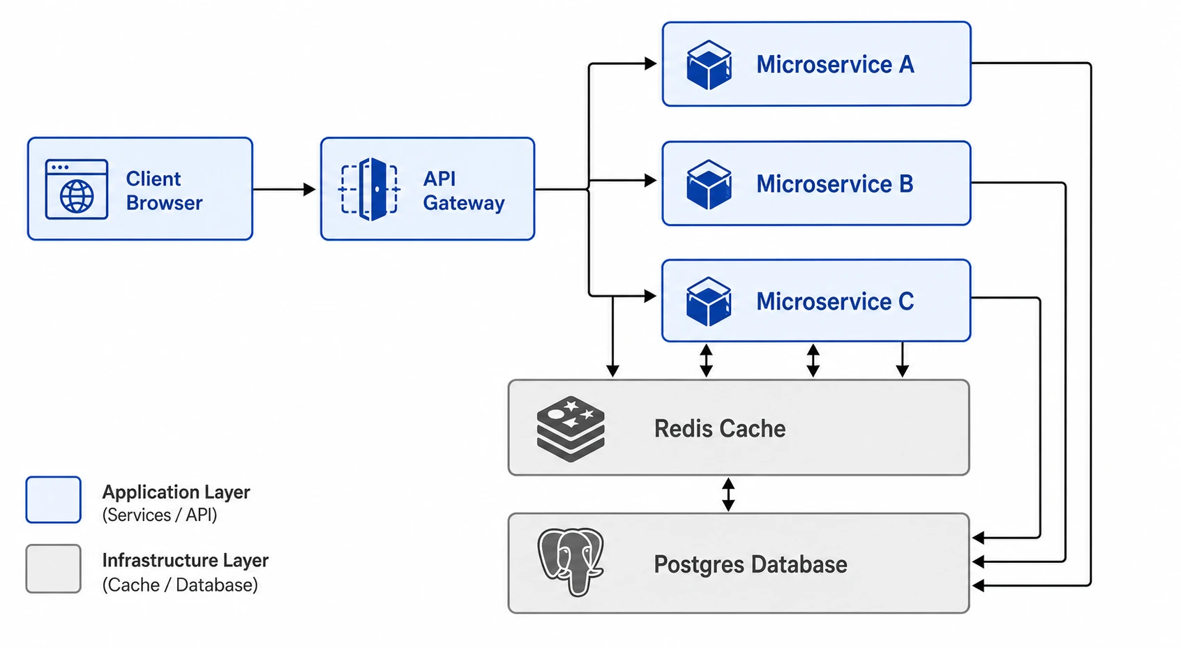 Software Architecture Diagram Generator
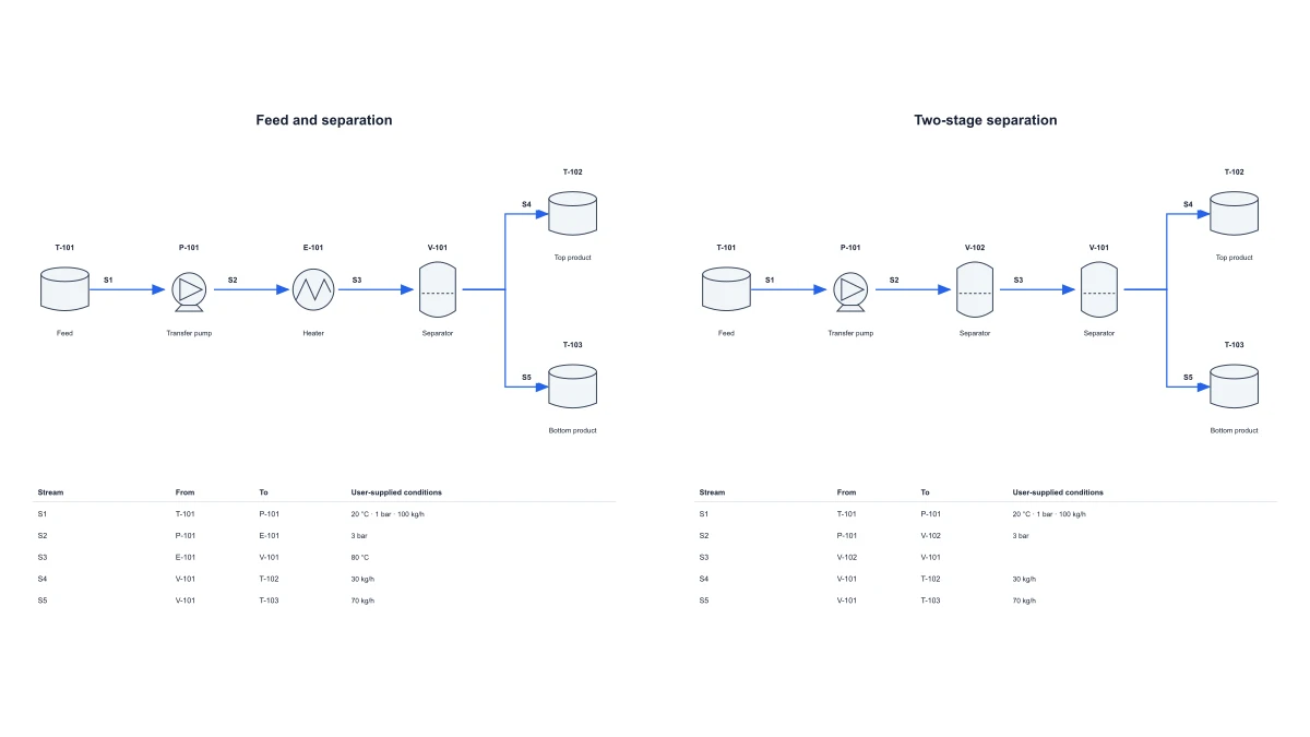 Chemical Process Flow Diagram Maker
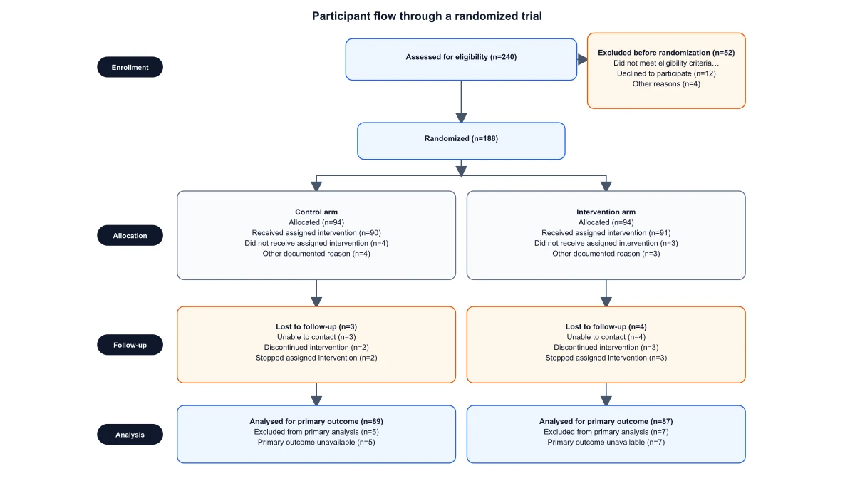 CONSORT Flow Diagram Generator
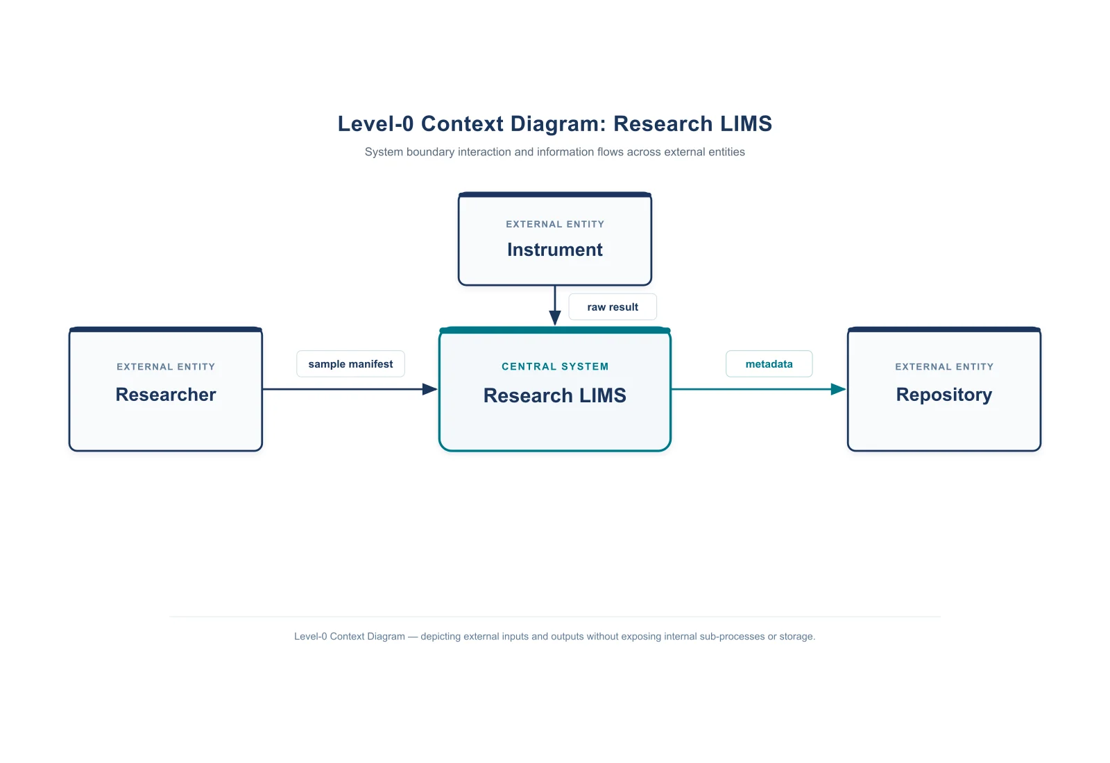 Context Diagram Creator
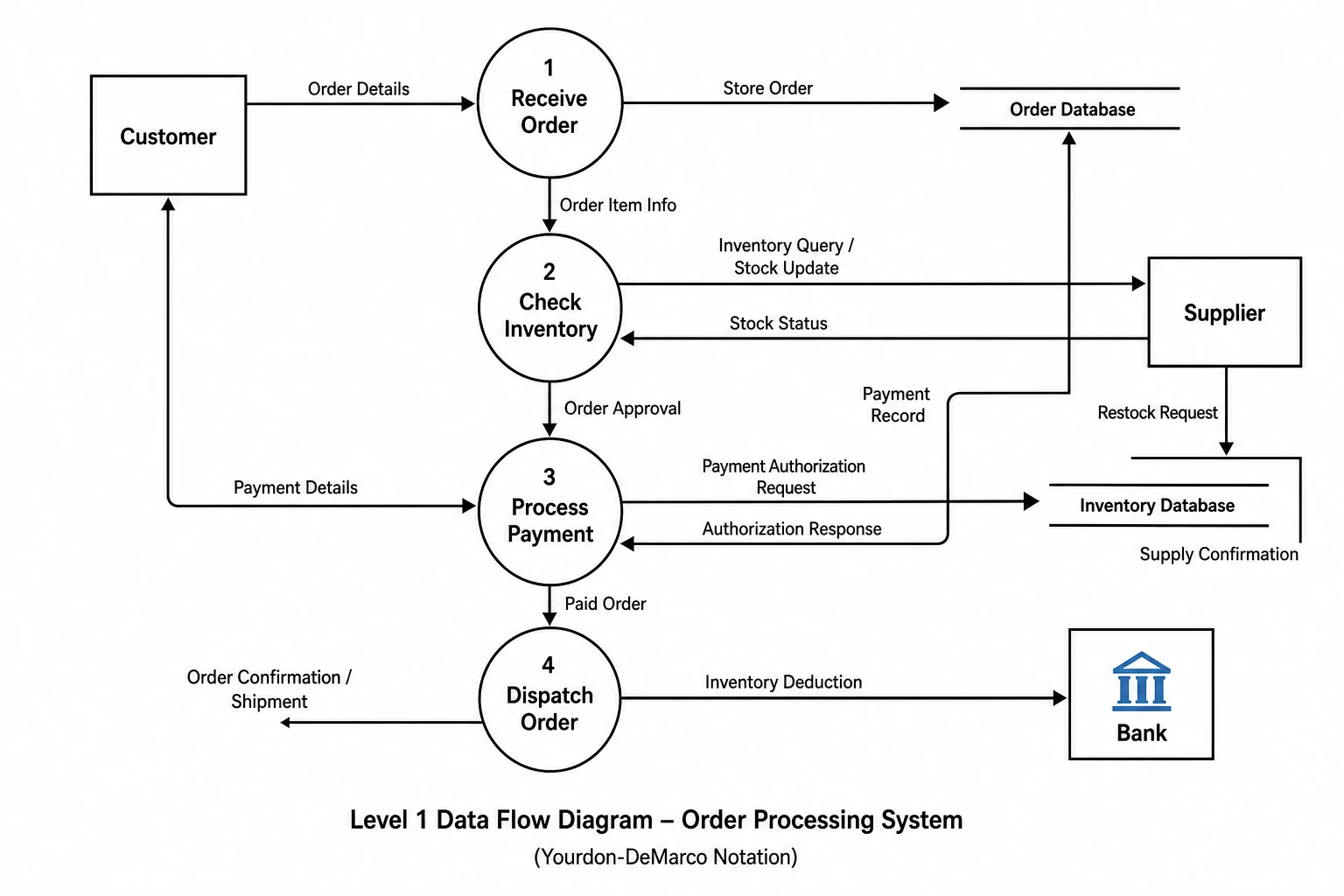 Data Flow Diagram Generator
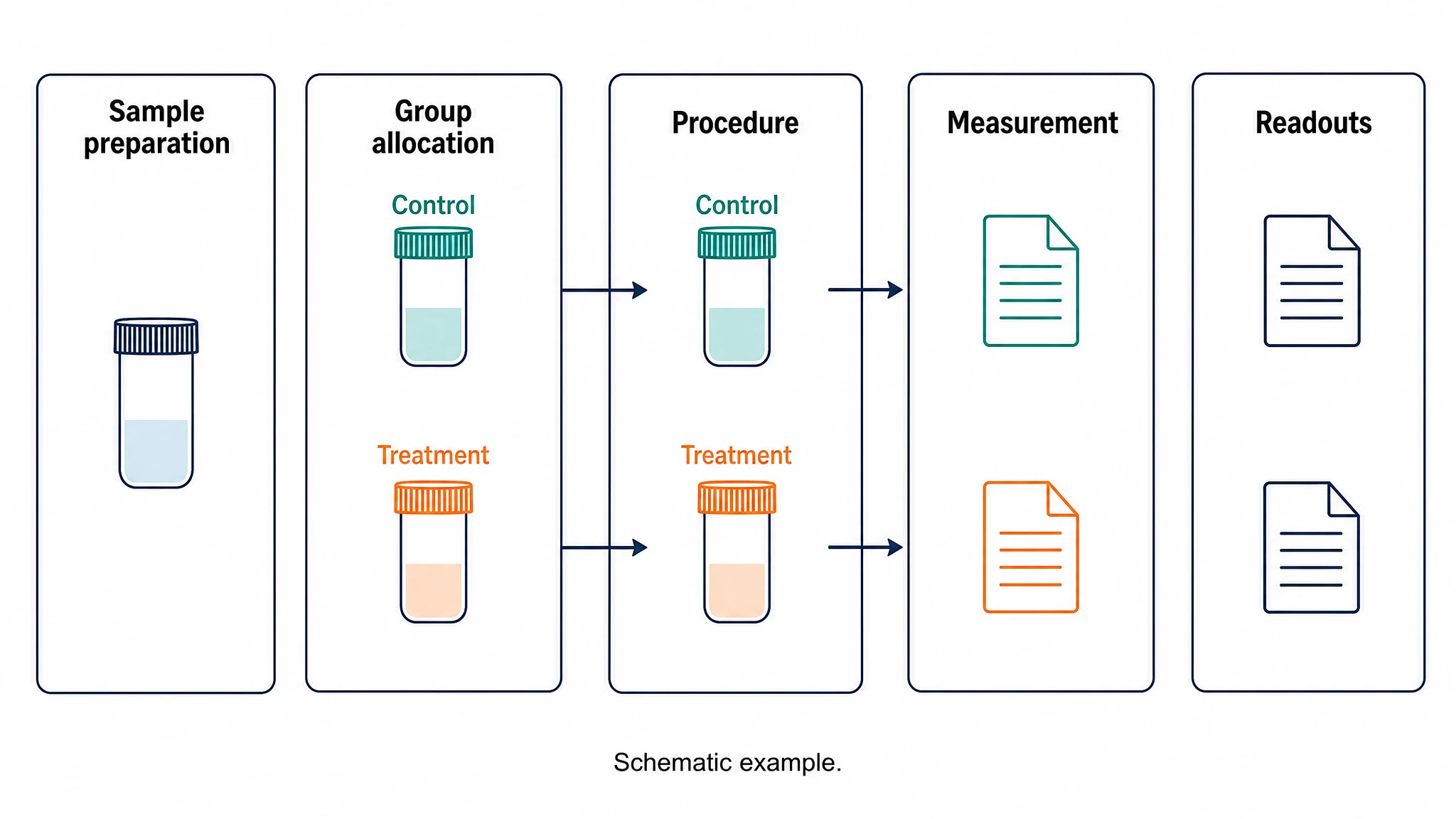 Experimental Workflow Diagram
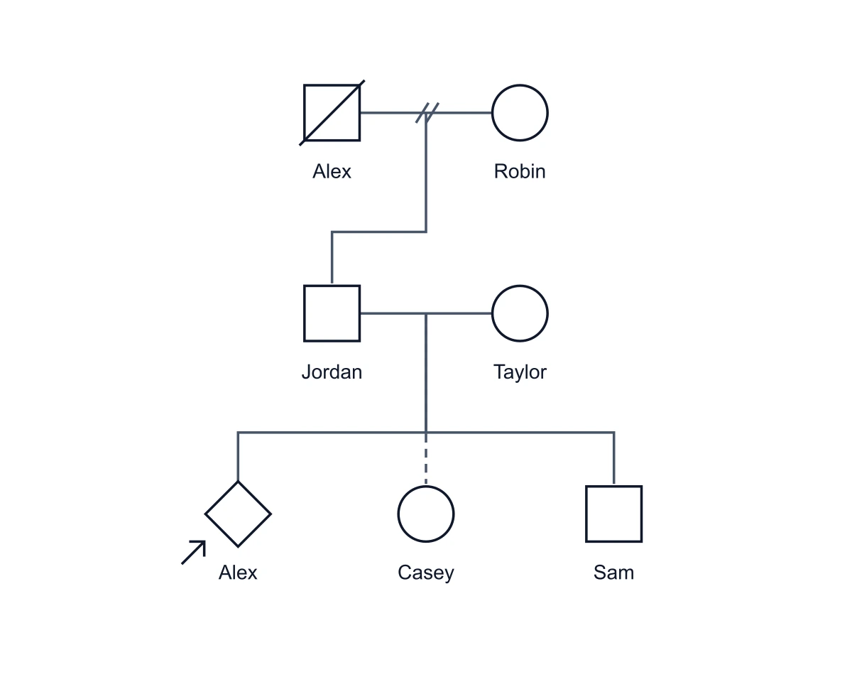 Genogram Maker
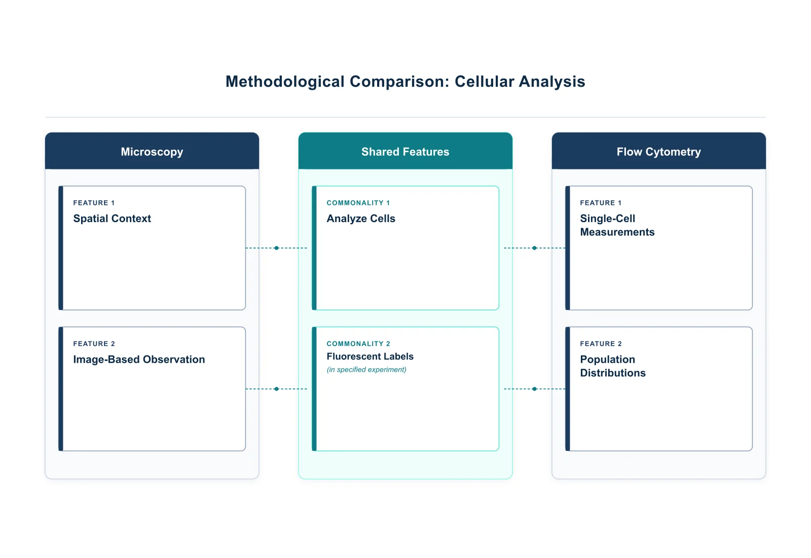 Graphic Organizer Generator
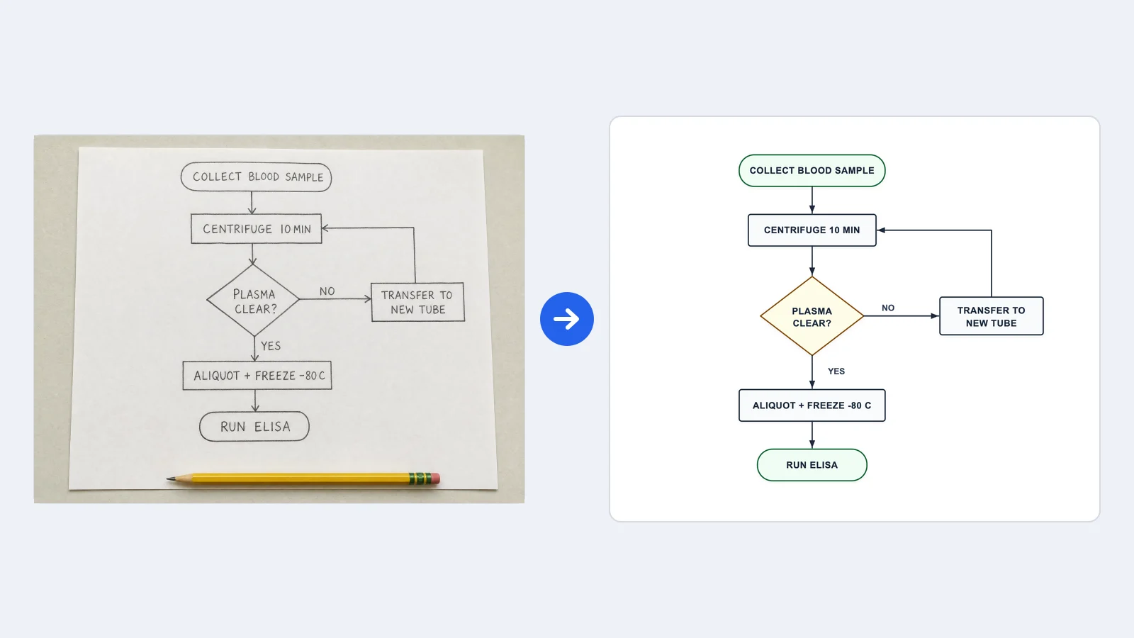 Image to Flowchart Converter
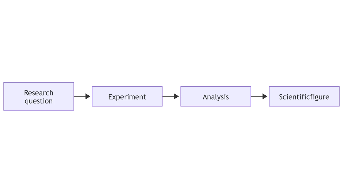 Mermaid to PNG Converter
 Network Diagram Generator
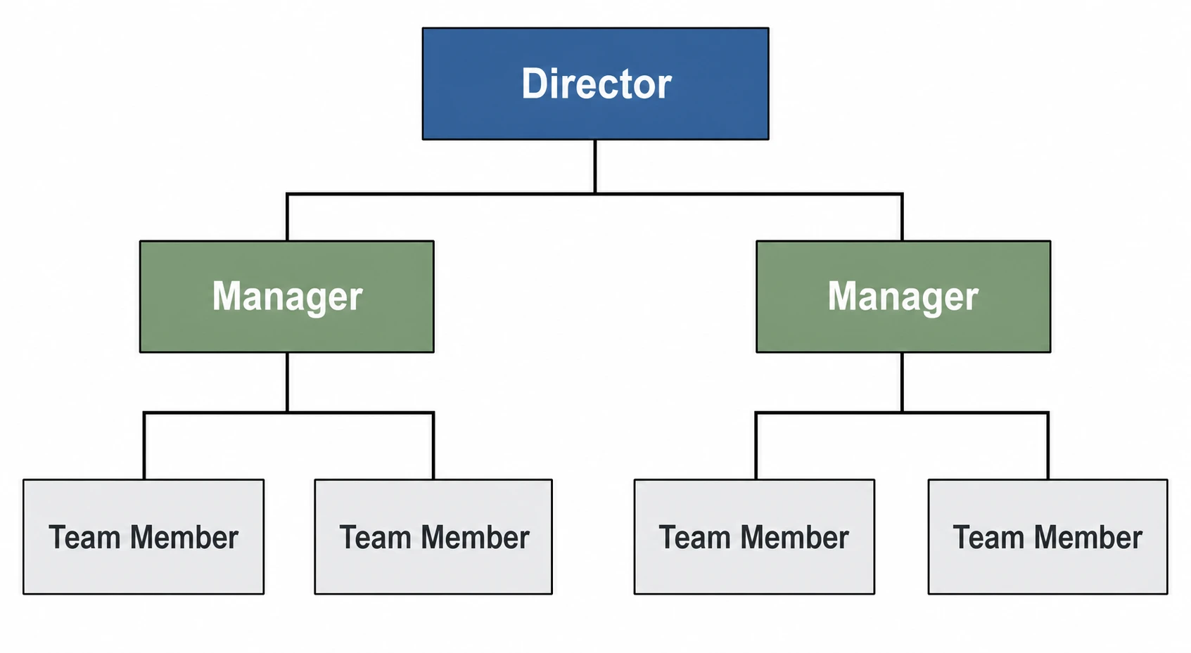 Org Chart Maker
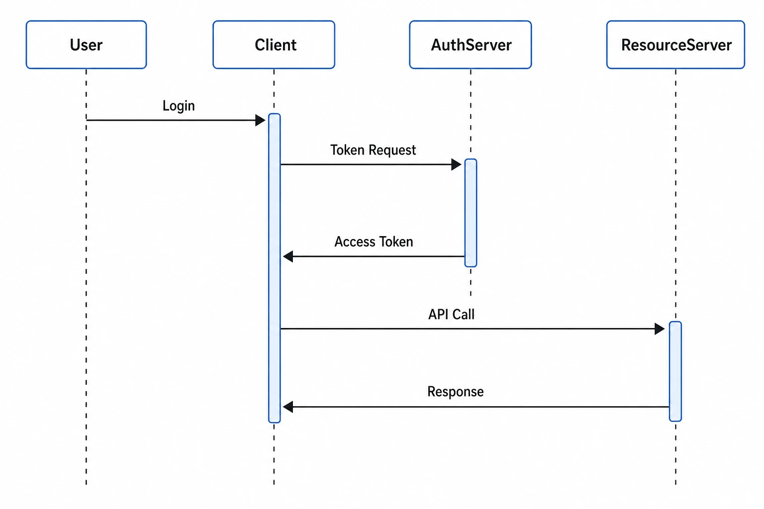 Sequence Diagram Generator
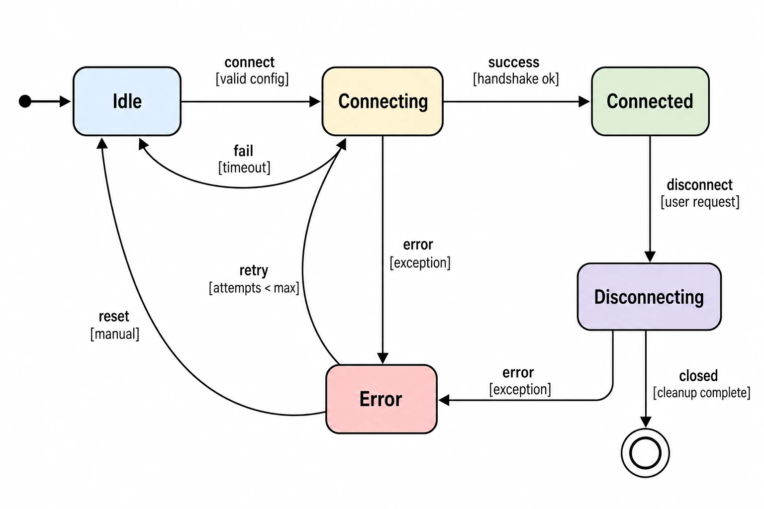 State Diagram Generator
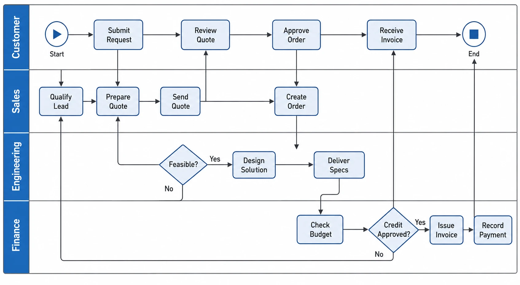 Swimlane Diagram Generator
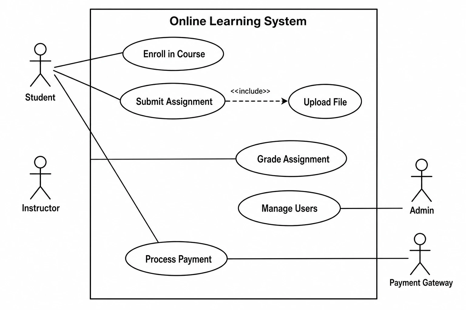 Use Case Diagram Generator
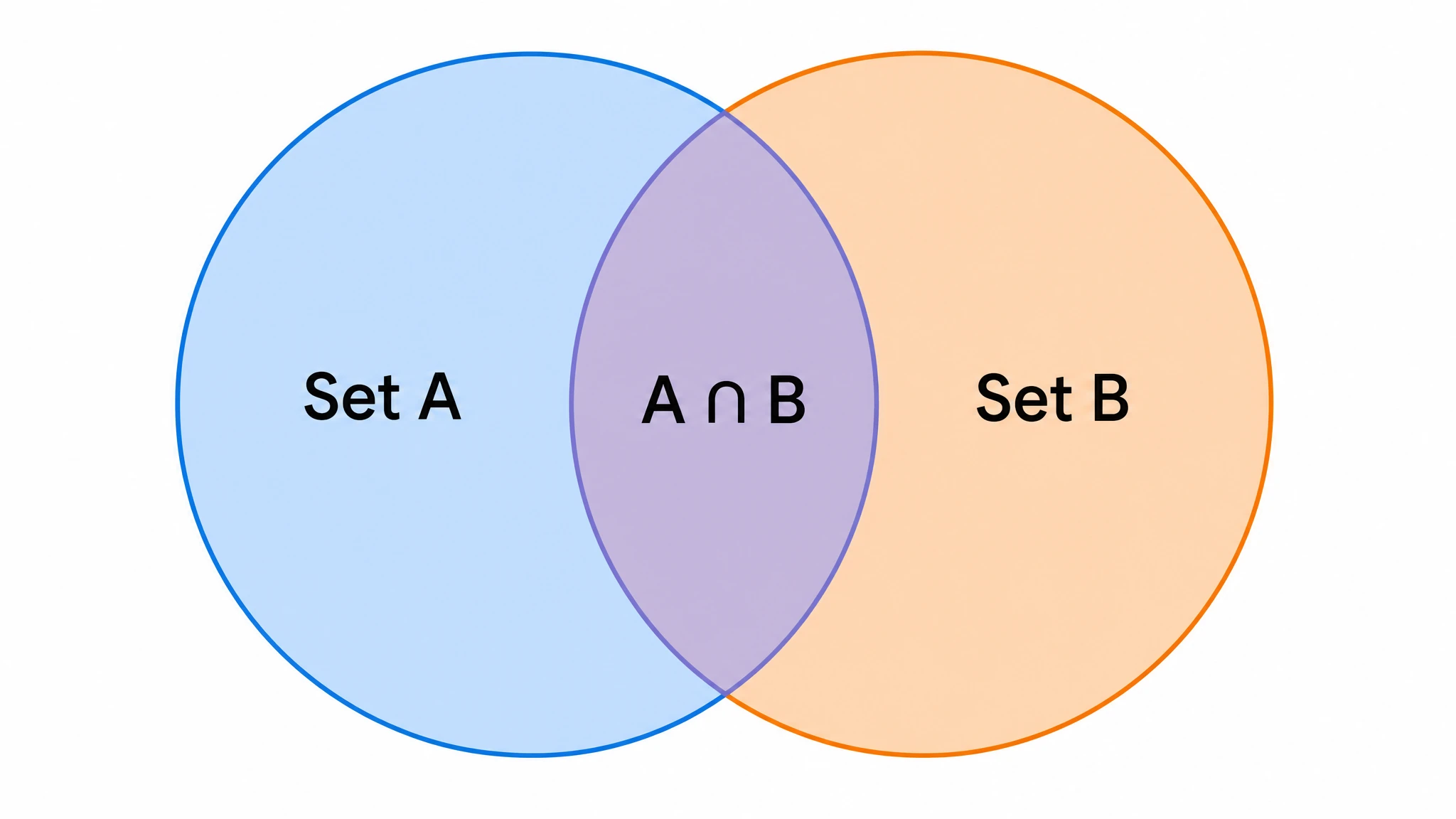 Venn Diagram Generator

Create with SciFig
Free to start · No credit card required · Built for researchers