Publication-ready template

96-Well Plate Diagram

Name: SciFig
Author: SciFig

A clean, editable 96-well plate diagram for mapping experiment layouts, plate setups, and assay conditions across all 96 wells in an 8x12 grid.

Editable SVGPublication-readyScientifically accurateFree to start

Use this template Edit this template

Editable 96 well plate diagram showing a standard 8x12 microplate layout with rows A to H and columns 1 to 12 and color-coded wells (Figure generated with SciFig)

Figure prompt

Core Subject (e.g., Cas9 protein cutting DNA)

Action / Details (e.g., Double strand break, detailed molecular view)

Start with 200 free credits|No credit card required

Get up to 400 free credits on day one when you join through an invite.

6 input modes · 6 publication stylesEvery text editable · Multimodal enhanceEditable PPTX · Layered SVG · 8K PNG / JPG

What is 96-Well Plate Diagram?

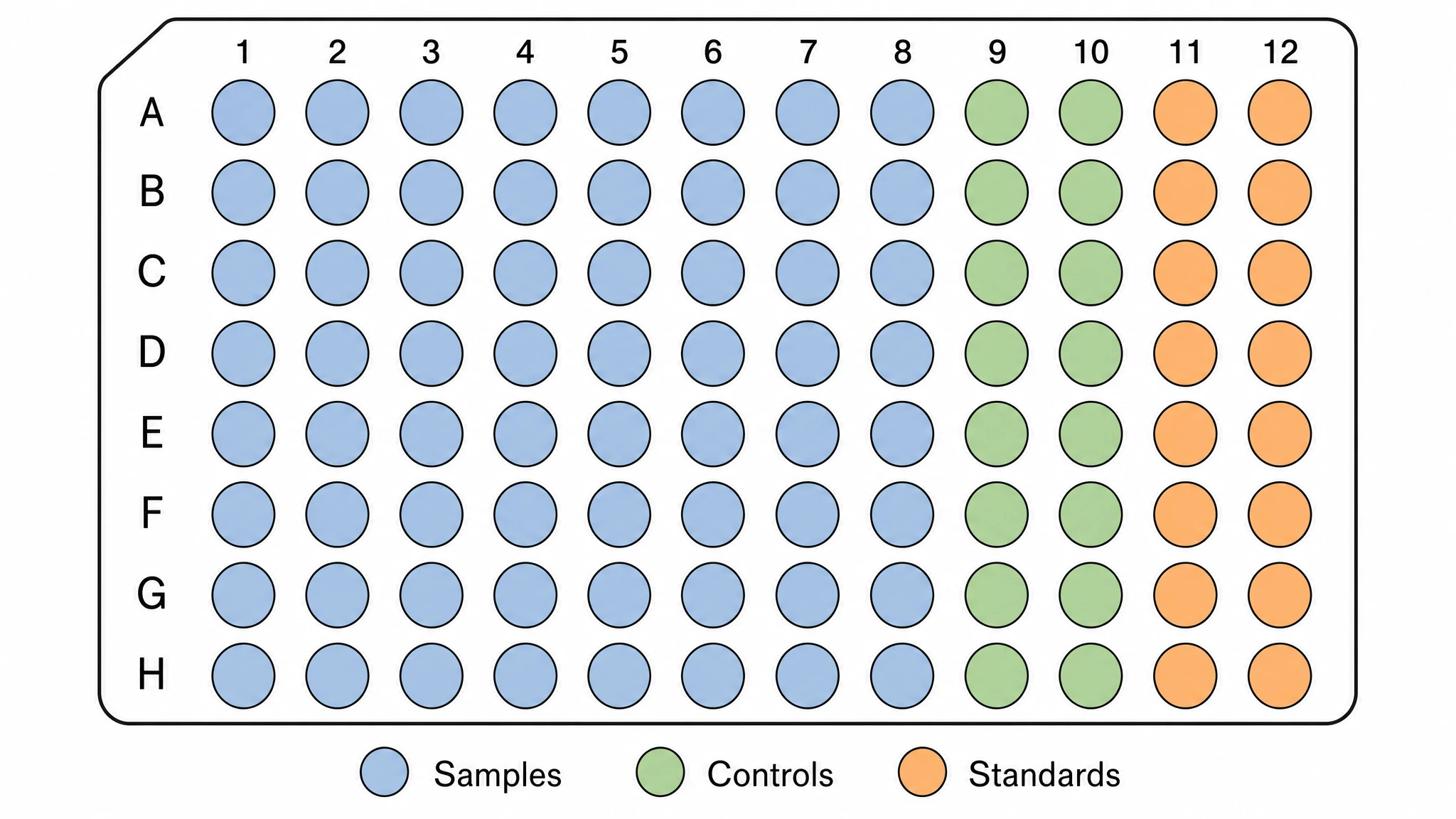
A 96-well plate diagram is a labeled map of a standard microplate, drawn as an 8x12 grid of 96 wells with rows lettered A to H and columns numbered 1 to 12. It is used to plan and record plate setups — which samples, controls, and replicates go in each well — so an assay runs without mix-ups. With SciFig you describe your microplate layout in plain language and generate a clean, editable 96-well plate template you can relabel and export.

Why plan the layout before you pipette

Every well is a pipetting decision. A map made in advance turns a multichannel run into a mechanical operation and removes the mid-assay improvisation where mix-ups happen.
Edge effects, evaporation and thermal gradients are positional artefacts. They can only be handled by a layout decision; no statistical correction after the fact recovers a plate that was laid out badly.
Randomising or block-balancing treatment positions stops plate position from confounding the treatment effect — the most common design flaw in plate-based screens.
Replicate structure has to be planned, not inferred. Three wells from one lysate is not n = 3, and the layout is where that distinction becomes explicit and auditable.
The analysis needs to know which addresses are blanks, standards and samples. A map that exists only in someone's head cannot be joined to the reader output.
Methods sections and supplementary figures need the actual layout; reconstructing it from a notebook months later is unreliable and often impossible.

What belongs on a complete plate map

Grid and addressing — eight rows (A to H) by twelve columns (1 to 12), 96 addresses from A1 to H12, drawn at the 9 mm pitch of the SBS footprint.
Sample wells — identity, treatment and concentration for each, with the direction of any dilution series stated explicitly rather than implied.
Blank wells — medium or assay buffer with no cells or analyte, used for background subtraction; run at least three and keep them off the perimeter.
Standard curve — a serial dilution, commonly seven or eight points plus a zero, in duplicate or triplicate; usually parked in the first one or two columns for ELISA and BCA-type assays.
Controls — untreated and vehicle wells (for example 0.1% DMSO), a positive control such as a known cytotoxin or a maximum-lysis well, and a negative control. These anchor the dynamic range and let you compute a Z' factor.
Replicates — technical replicates within the plate versus biological replicates across plates or independent cultures, marked differently so the analysis does not conflate them.
Plate format notes — flat, round or V-bottom wells, and the optical type (clear for absorbance, black for fluorescence, white for luminescence), since these determine which readings are even valid.

Assays this layout is built for

Sandwich ELISA, with a seven-point standard curve in duplicate and blank wells for background subtraction.
Cell viability and cytotoxicity assays (MTT, CCK-8, resazurin) with an eight-point half-log dose series and vehicle plus maximum-lysis controls.
qPCR run in 96-well blocks, where the map has to carry no-template and no-reverse-transcriptase controls alongside samples.
Bacterial growth curves and MIC checkerboards read kinetically at OD600, where perimeter evaporation over a long run is a real source of error.
Compound-library screening, where positive and negative control columns are used to compute the Z' factor that qualifies each plate.
Protein quantification by BCA or Bradford, with a BSA standard series and sample wells read against it.

What a labelled microplate map does for an assay, from the blank grid to the finished record.

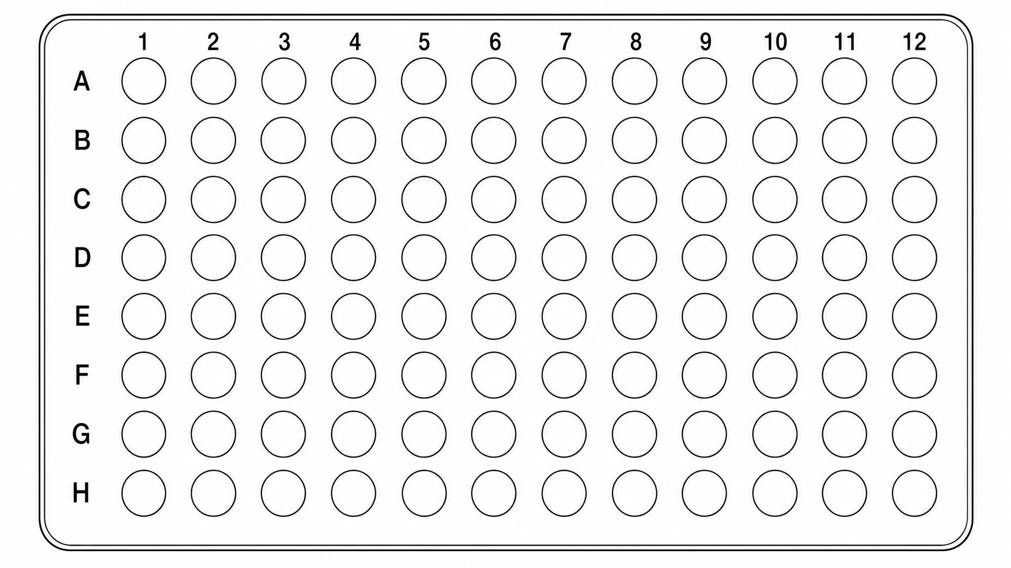
Start from the blank 8x12 grid

The standard microplate follows the SBS footprint of 127.76 x 85.48 mm with a 9 mm well pitch, giving eight rows and twelve columns. A blank grid is the working surface: you fill it in before touching a pipette, not afterwards. Well capacity is typically around 360 microlitres with 100-200 microlitres of working volume, so the map should record volumes as well as identities.

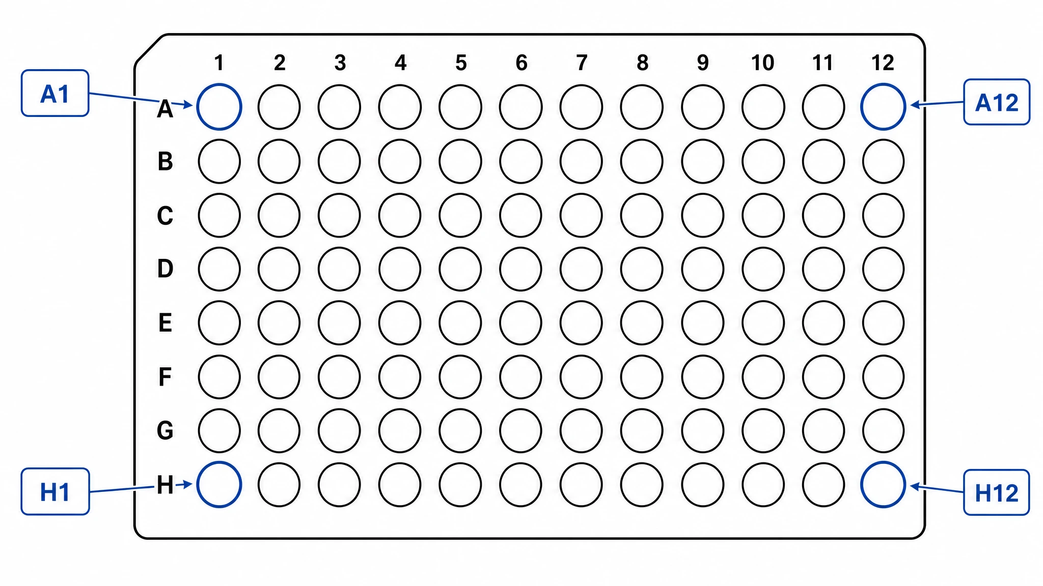
Coordinates that match your plate reader export

Rows are lettered A to H and columns numbered 1 to 12, so every well has a unique address from A1 to H12. Readers export in the same coordinate space, usually as row-major or column-major CSV, which means a map drawn with correct addressing can be joined straight to raw absorbance or fluorescence values with no manual re-keying. Label the axes exactly as the instrument does.

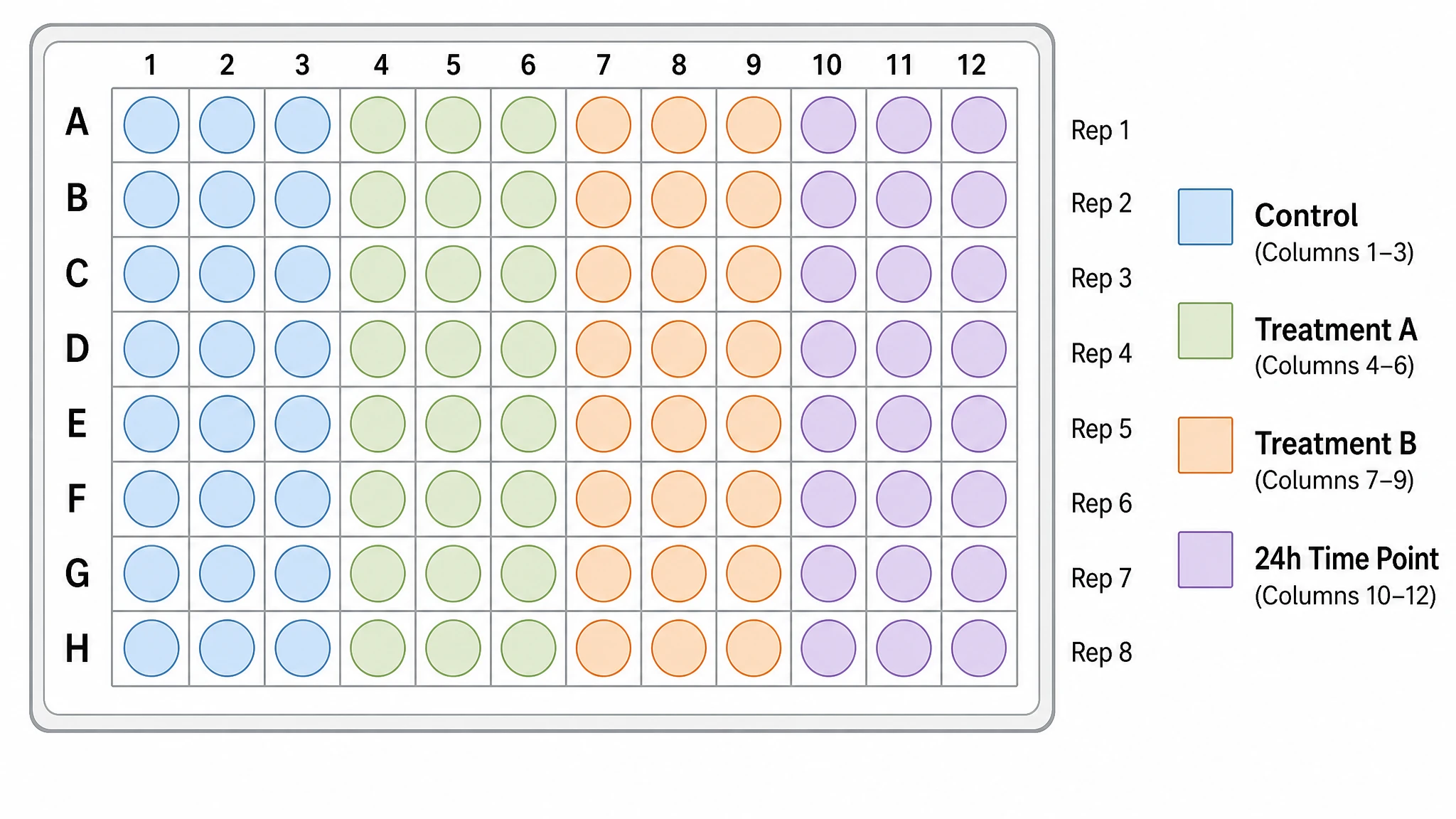
Placing conditions to defeat edge effects

Perimeter wells evaporate faster and sit at a different temperature, biasing the outermost ring. Two accepted mitigations: fill the border with buffer or PBS and use only the inner 60 wells, or randomise treatments across positions so a spatial gradient is spread across all conditions instead of being confounded with one. Never run a dose series so that concentration increases monotonically along a column.

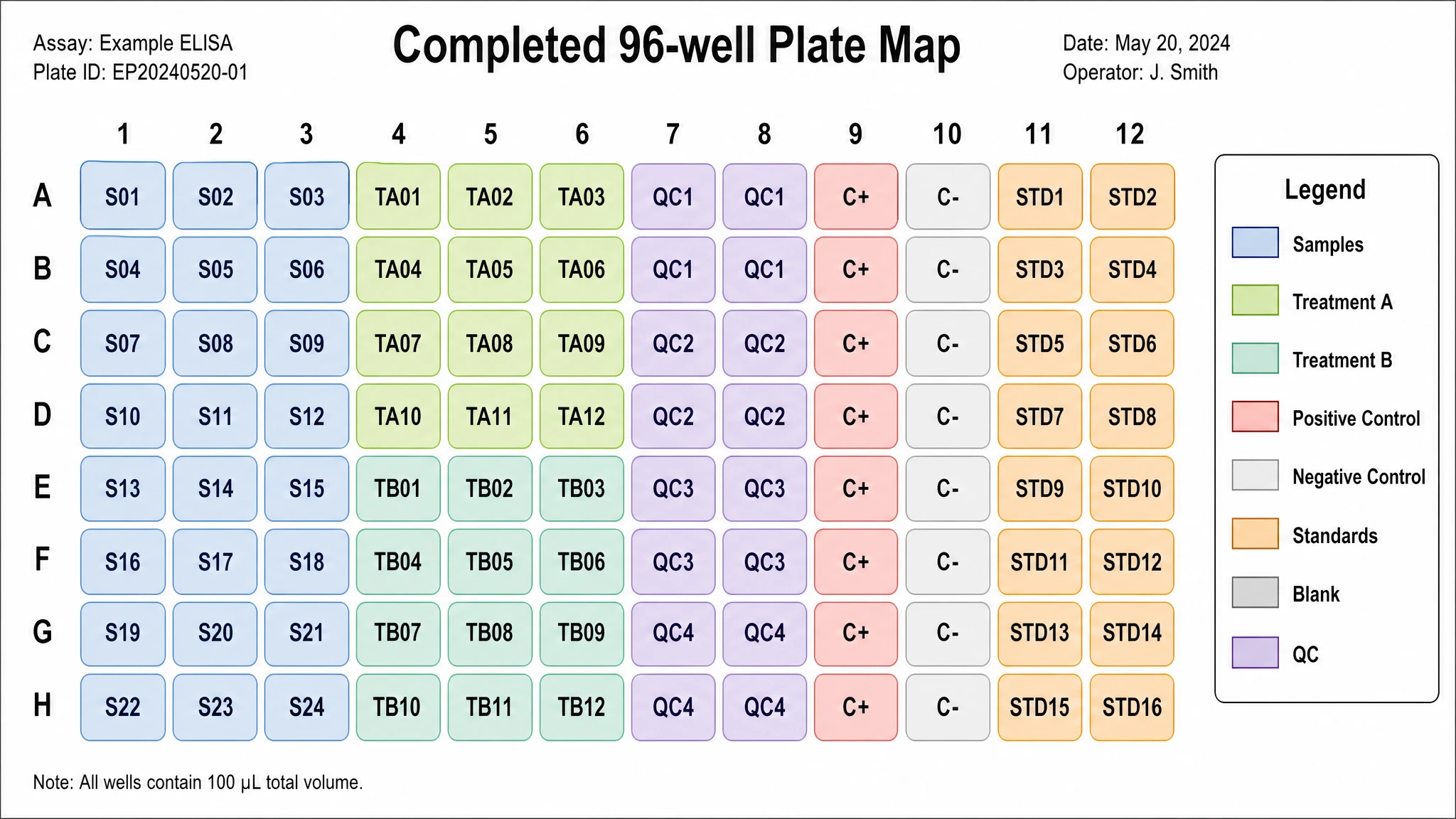
The finished map as an assay record

A completed layout records sample identity, treatment, concentration and replicate class for every well. Distinguish technical replicates (one lysate pipetted into three wells) from biological replicates (independent cultures or animals) — only the latter carries degrees of freedom into your statistics. Keep blanks and standard-curve wells on the map too, since the analysis script needs to know which addresses to subtract and which to fit.